Optimal Estimation of Distinct Elements in Streaming Data
This paper presents an optimal approach to estimating the number of distinct elements (F0) from a long string of at most n distinct characters within a limited memory setting. We aim to provide a solution with a single pass over the data while ensuring fast update times and using randomized algorithms to achieve approximate results with high probability. We explore various historical algorithms, their complexities, and establish both upper and lower bounds on memory usage and update time, culminating in a significant improvement over existing methods.


Optimal Estimation of Distinct Elements in Streaming Data
E N D
Presentation Transcript
Estimating Distinct Elements, Optimally David Woodruff IBM Based on papers with Piotr Indyk, Daniel Kane, and Jelani Nelson
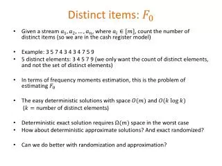
Problem Description • Given a long string of at most n distinct characters, count the number F0 of distinct characters • See characters one at a time • One pass over the string • Algorithms must use small memory and fast update time • too expensive to store set of distinct characters • algorithms must be randomized and settle for an approximate solution: output F 2 [(1-²)F0, (1+²)F0] with, say, good constant probability
Algorithm History • Flajolet and Martin introduced problem, FOCS 1983 • O(log n) space for fixed ε in random oracle model • Alon, Matias and Szegedy • O(log n) space/update time for fixed ε with no oracle • Gibbons and Tirthapura • O(ε-2 log n) space and O(ε-2) update time • Bar-Yossef et al • O(ε-2 log n) space and O(log 1/ε) update time • O(ε-2log log n + log n) space and O(ε-2) update time, essentially • Similar space bound also obtained by Flajolet et al in the random oracle model • Kane, Nelson and W • O(ε-2+ log n) space and O(1) update and reporting time • All time complexities are in unit-cost RAM model
Lower Bound History • Alon, Matias and Szegedy • Any algorithm requires Ω(log n) bits of space • Bar-Yossef • Any algorithm requires Ω(ε-1) bits of space • Indyk and W • If ε > 1/n1/9, any algorithm needs Ω(ε-2) bits of space • W • If ε > 1/n1/2, any algorithm needs Ω(ε-2) bits of space • Jayram, Kumar and Sivakumar • Simpler proof of Ω(ε-2) bound for any ε > 1/m1/2 • Brody and Chakrabarti • Show above lower bounds hold even for multiple passes over the string Combining upper and lower bounds, the complexity of this problem is: Θ(ε-2+ log n) space and Θ(1) update and reporting time
Outline for Remainder of Talk • Proofs of the Upper Bounds • Proofs of the Lower Bounds
Hash Functions for Throwing Balls • We consider a random mapping f of B balls into C containers and count the number of non-empty containers • The expected number of non-empty containers is C – C(1-1/C)B • If instead of the mapping f, we use an O(log C/ε)/log log C/ε – wise independent mapping g, then • the expected number of non-empty containers under g is the same as that under f, up to a factor of (1 ± ε) • Proof based on approximate inclusion-exclusion • express 1 – (1-1/C)B in terms of a series of binomial coefficients • truncate the series at an appropriate place • use limited independence to handle the remaining terms
Fast Hash Functions • Use hash functions g that can be evaluated in O(1) time. • If g is O(log C/ε)/(log log C/ε)-wise independent, the natural family of polynomial hash functions doesn’t work • We use theorems due to Pagh, Pagh, and Siegel that construct k-wise independent families for large k, and allow O(1) evaluation time • For example, Siegel shows: • Let U = [u] and V = [v] with u = vc for a constant c > 1, and suppose the machine word size is Ω(log v) • Let k = vo(1) be arbitrary • For any constant d > 0 there is a randomized procedure that constructs a k-wise independent hash family H from U to V that succeeds with probability 1-1/vd and requires vd space. Each h 2 H can be evaluated in O(1) time • Can show we have sufficiently random hash functions that can be evaluated in O(1) time and represented with O(ε-2+ log n) bits of space
Algorithm Outline • Set K = 1/ε2 • Instantiate a lg n x K bitmatrix A, initializing entries of A to 0 • Pick random hash functions f: [n]->[n] and g: [n]->[K] • Obtain a constant factor approximation R to F0 somehow • Update(i): Set A1, g(i) = 1, A2, g(i) = 1, …, Alsb(f(i)), g(i) = 1 • Estimator: Let T = |{j in [K]: Alog (16R/K), j = 1}| Output (32R/K) * ln(1-T/K)/ln(1-1/K)
Space Complexity • Naively, A is a lg n x K bitmatrix, so O(ε-2 log n) space • Better: for each column j, store the identity of the largest row i(j) for which Ai, j = 1. Note if Ai,j = 1, then Ai’, j = 1 for all i’ < i • Takes O(ε-2 log log n) space • Better yet: maintain a “base level” I. For each column j, store max(i(j) – I, 0) • Given an O(1)-approximation R to F0 at each point in the stream, set I = log R • Don’t need to remember i(j) if i(j) < I, since j won’t be used in estimator • For the j for which i(j) ¸ I, about 1/2 such j will have i(j) = I, about one fourth such j will have i(j) = I+1, etc. • Total number of bits to store offsets is now only O(K) = O(ε-2) with good probability at all points in the stream
The Constant Factor Approximation • Previous algorithms state that at each point in the stream, with probability 1-δ, the output is an O(1)-approximation to F0 • The space of such algorithms is O(log n log 1/δ). • Union-bounding over a stream of length m gives O(log n log m) total space • We achieve O(log n) space, and guarantee the O(1)-approximation R of the algorithm is non-decreasing • Apply the previous scheme on a log n x log n/(log log n) matrix • For each column, maintain the identity of the deepest row with value 1 • Output 2i, where i is the largest row containing a constant fraction of 1s • We repeat the procedure O(1) times, and output the median of the estimates • Can show the output is correct with probability 1- O(1/log n) • Then we use the non-decreasing property to union-bound over O(log n) events • We only increase the base level every time R increases by a factor of 2 • Note that the base level never decreases
Running Time • Blandford and Blelloch • Definition: a variable length array (VLA) is a data structure implementing an array C1, …, Cn supporting the following operations: • Update(i, x) sets the value of Ci to x • Read(i) returnsCi The Ci are allowed to have bit representations of varying lengths len(Ci). • Theorem: there is a VLA using O(n + sumi len(Ci)) bits of space supporting worst case O(1) updates and reads, assuming the machine word size is at least log n • Store our offsets in a VLA, giving O(1) update time for a fixed base level • Occasionally we need to update the base level and decrement offsets by 1 • Show base level only increases after Θ(ε-2) updates, so can spread this work across these updates, so O(1) worst-case update time • Copy the data structure, use it for performing this additional work so it doesn’t interfere with reporting the correct answer • When base level changes, switch to copy • For O(1) reporting time, maintain a count of non-zero containers in a level
Outline for Remainder of Talk • Proofs of the Upper Bounds • Proofs of the Lower Bounds
1-Round Communication Complexity Alice: Bob: What is f(x,y)? input x input y • Alice sends a single, randomized message M(x) to Bob • Bob outputs g(M(x), y) for a randomized function g • g(M(x), y) should equal f(x,y) with constant probability • Communication cost CC(f) is |M(x)|, maximized over x and random bits • Alice creates a string s(x), runs a randomized algorithm A on s(x), and • transmits the state of A(s(x)) to Bob • Bob creates a string s(y), continues A on s(y), thus computing A(s(x)◦s(y)) • If A(s(x)◦s(y)) can be used to solve f(x,y), then space(A) ¸ CC(f)
The Ω(log n) Bound • Consider equality function: f(x,y) = 1 if and only if x = y for x, y 2 {0,1}n/3 • Well known that CC(f) = Ω(log n)for(n/3)-bit stringsxandy • Let C: {0,1}n/3 -> {0,1}nbe an error-correcting code with all codewords of Hamming weight n/10 • If x = y, then C(x) = C(y) • If x != y, then¢(C(x), C(y)) = Ω(n) • Let s(x) be any string on alphabet size n with i-th character appearing in s(x) if and only if C(x)i = 1. Similarly define s(y) • If x = y, then F0(s(x)◦s(y)) = n/10. Else, F0(s(x)◦s(y)) = n/10 + Ω(n) • A constant factor approximation to F0solves f(x,y)
The Ω(ε-2) Bound • Let r = 1/ε2. Gap Hamming promise problem for x, y in {0,1}r • f(x,y) = 1 if ¢(x,y) > 1/(2ε-2) • f(x,y) = 0 if ¢(x,y) < 1/(2ε-2) - 1/ε • Theorem: CC(f) = Ω(ε-2) • Can prove this from the Indexing function • Alice has w 2 {0,1}r, Bob has i in {1, 2, …, r}, output g(w, i) = wi • Well-known that CC(g) = Ω(r) • Proof: CC(f) = Ω(r), • Alice sends the seed r of a pseudorandom generator to Bob, so the parties have common random strings zi, …, zr2 {0,1}r • Alice sets x = coordinate-wise-majority{zi | wj = 1} • Bob sets y = zi • Since the ziare random, if xj = 1, then by properties of majority, with good probability ¢f(x,y) < 1/(2ε-2) - 1/ε, otherwise likely that¢f(x,y) > 1/(2ε-2) • Repeat a few times to get concentration
The Ω(ε-2) Bound Continued • Need to create strings s(x) and s(y) to have F0(s(x)◦s(y)) decidewhether¢(x,y) > 1/(2ε-2) or ¢(x,y) < 1/(2ε-2) - 1/ε • Let s(x) be a string on n characters where character i appears if and only if xi = 1. Similarly define s(y) • F0(s(x)◦s(y)) = (wt(x) + wt(y) + ¢(x,y))/2 • Alice sends wt(x) to Bob • A calculation shows a (1+ε)-approximation to F0(s(x)◦s(y)), together with wt(x) and wt(y), solves the Gap-Hamming problem • Total communication is space(A) + log 1/ε = Ω(ε-2) • It follows that space(A) = Ω(ε-2)
Conclusion Combining upper and lower bounds, the streaming complexity of estimating F0 up to a (1+ε) factor is: Θ(ε-2+ log n) bits of space and Θ(1) update and reporting time • Upper bounds based on careful combination of efficient hashing, • sampling and various data structures • Lower bounds come from 1-way communication complexity