Investment Tools – Probability
470 likes | 493 Vues
Learn about the properties of probability including intersection, union, joint probabilities, conditional probability, and statistical independence. Explore the calculation of expected value, variance, and standard deviation.

Investment Tools – Probability
E N D
Presentation Transcript
SASF CFA Quant. Review Investment Tools – Probability
Probability • A random variable is a quantity whose outcome is uncertain. • Two defining properties of Probability. • Probability of any event E is a number between 0 and 1, p(E). • Sum of the probabilities of any list of mutually exclusive and exhaustive events equals 1. • Mutually exclusive = one and only one event can occur at any time. • Exhaustive = one of the events must occur, jointly cover all possible outcomes. • Empirical probability - probability of an event occurring is estimated from data, usually in the form of a relative frequency. • A priori probability - probability of an event is deduced by reasoning about the structure of the problem itself. • Subjective probability - probability of an event is based on a personal assessment without reference to any particular data.
Visualizing Sample Space 1. Listing • S = {Head, Tail} 2. Contingency Table 3. Decision Tree Diagram
Outcome (Count, Total % Shown Usually) SimpleEvent (Head on1st Coin) S = {HH, HT, TH, TT} Sample Space Contingency Table Experiment: Toss 2 Coins. Note Faces. nd 2 Coin st Head Tail 1 Coin Total Head HH HT HH, HT Tail TH TT TH, TT Total HH, TH HT, TT S
Tree Diagram Experiment: Toss 2 Coins. Note Faces. H HH H T HT Outcome H TH T T TT S = {HH, HT, TH, TT} Sample Space
Probabilities for Two Dice Second Die First Die
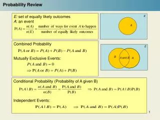
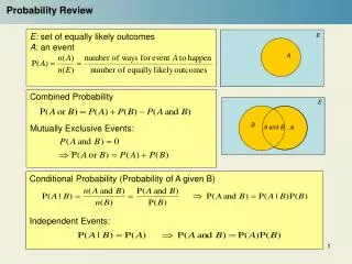
Forming Compound Events 1. Intersection • Outcomes in Both Events A and B • ‘AND’ Statement • Symbol (i.e., A B) 2. Union • Outcomes in Either Events A or B or Both • ‘OR’ Statement • Symbol (i.e., A B)
Joint Probabilities for Two Dice Second Die What is the Probability of throwing a Seven with the two Dice? First Die Answer: Count the combinations that yield 7 and add the individual probabilities to find the probability of the event, A, “Rolling a seven” P(A) = P(AB1) + P(A B2) + P(AB3) +…+ P(A B6) = 6/36 = 1/6
Addition Rule 1. Used to Get Compound Probabilities for Union of Events: P(A OR B) = P(A B) = P(A) + P(B) - P(A B) 2. For Mutually Exclusive Events: P(A OR B) = P(A B) = P(A) + P(B)
Addition Rule for Probabilities What is the Probability of throwing at least one die showing 1 with the two Dice? Second Die Answer: Count the combinations that have one die with 1 and add the individual probabilities OR use the Addition Rule for probabilities. P(AB) = P(A) + P(B) - P(A B) = 1/6 + 1/6 -1/36 = 11/36 First Die
Addition Rule - Again What is the Probability of throwing a four or higher on either the first or second die? Second Die Answer: Count the combinations that have one die with 4 or greater & add the individual probabilities OR use the Addition Rule for probabilities. P(AB) = P(A) + P(B) - P(A B) = 1/2 + 1/2 -1/4 = 3/4 First Die
Conditional Probability Conditional Probability: • Probability that one Event will occur Given that Another Event has already occurred. To calculate a Conditional probability – • Revise Original Sample Space to Account for New Information • Eliminates Certain Outcomes Result: • P(A |B) = P(A and B) P(B)
Conditional Probability What is the Probability of throwing at least an 8 if the first die is a 4? Second Die Answer: Note we know we are in the row associated with a 4 for the first die. There are only 3 ways of the possible six outcomes for the second die that yield a sum 8. Hence P(A|B) = = P(AB)/P(B) = (3/36)/(6/36) =.5 First Die
Statistical Independence 1. Event Occurrence Does Not Affect Probability of Another Event • Toss first die, what does its outcome tell you about the likely results in tossing the second die? • Answer: Nothing. The two die are independent 2. Causality Not Implied 3. Tests For Statistical Independence • P(A | B) = P(A) • P(A and B) = P(A)*P(B)
Multiplication Rule 1. Used to Get Compound Probabilities for Intersection of Events • Called Joint Events 2. P(A and B) = P(A B) = P(A)*P(B|A) = P(B)*P(A|B) 3. For Independent Events:P(A and B) = P(A B) = P(A)*P(B)
Multiplication Rule with Independence What is the Probability of throwing “snake eyes” i.e. a 1 on each die? Answer: The result on the first die is independent of the second die. We use The multiplication rule to find prob. of A and B Hence P(AB) = = P(A)*P(B) = (1/6)*(1/6) = (1/36) Second Die First Die
Discrete R.V.’s - Summary Measures Expected Value • Mean of Probability Distribution • Weighted Average of All Possible Values X = E(X)= Xi P(Xi) = p(X1) X1+ p(X2) X2+ … + p(Xn) Xn Variance • Weighted Average Squared Deviation about Mean X2 = E[ (Xi-X(Xi-XP(Xi) = p(X1)(X1- X)2 + p(X2 )(X2- X)2 + … + p(Xn) )(Xn- X)2 Standard deviation • Square root of the variance. Measure of risk shows dispersion of possible outcomes around expected level of outcomes.
Mean/Variance Calculation Table 2 2 X P(X ) X P(X ) X - (X - ) X X ( - ) P( ) i i i i i i i i 2 Total X X X P(X ) ( - ) P( ) i i i i
Asset Expected Return & Risk • Calculate the Expected Returns of alternative assets. • Rki= Return to Asset k if Event i occurs • P(Rki) = Probability Event i occurs.
Calculating ER and Risk • Can use the previous table to calculate ER and variance (risk) for each asset. • Show calculations for Asset A below. ERA = 9.1% A = 3.56% ERA/A = 2.55
Covariance • Covariance between two random variables X and Y is defined as • A negative covariance between X and Y means that when X is above its mean its is likely that Y is below its mean value. • If the covariance of the two random variables is zero then on average the values of the two variables are unrelated. • A positive covariance between X and Y means that when X is above its mean its is likely that Y is above its mean value. • Covariance of a random variable with itself, its own covariance, is equal to its variance.
Correlation • Correlation between two random variables X and Y measured as: • Correlation takes on values between –1 and +1. Correlation is a standardized measure of how two random variables move together, i.e. correlation has no units associated with it. • A correlation of 0 means there is no straight-line (linear) relationship between the two variables. • Increasingly positive (negative) correlations indicate an increasingly strong positive (negative) linear relationship between the variables. • When the correlation equals 1 (-1) there is a perfect positive (negative) linear relationship between the two variables.
Portfolio Probability Calculations Portfolio consisting of two assets A and B, wA invested in A. Asset A has expected return rA and variance s2A. Asset B has expected return rB and variance s2B. The correlation between the two returns is rAB. Portfolio Expected Return: E(rp) = wA rA + (1-wA )rB Portfolio Variance: or
28. The probability that two or more events will happen concurrently is: A. joint probability. B. multiple probability. C. concurrent probability. D. conditional probability. Exam Questions on Probability
24. An analyst developed the following probability distribution of the rate of return for a common stock: Scenario Probability Rate of return 1 0.25 0.08 2 0.50 0.12 3 0.25 0.16 The standard deviation of the rate of return is closest to: A. 0.0200. B. 0.0267. C. 0.0283. D. 0.0400. To calculate standard deviation must first calculate expected value, mean, of the rate of return. = [.25 x .08 + .5 x .12 + .25 x .16] = 0.12 Calculate variance as probability-weighted squared deviations of values from expected value. s2 = .25[.08 - .12]2 + .5[.12 - .12]2 + .25[.16 - .12]2 = 0.0008 Finally calculate standard deviation as square root of variance. s = SQRT(0.0008) = 0.02828 Exam Question on Expected Values
Probability distribution specifies the probabilities of the possible outcomes of a random variable. Discrete random variable can take on at most a countable number of possible values, such as coin flip or rolling dice. Continuous random variable can take on an uncountable (infinite) number of possible values, such as asset returns or temperatures. Probability function specifies the probability that the random variable takes on a specific value: P(X = x). Two Key Properties of a Probability Function. 0 ≤ p(x) ≤ 1 because a probability lies between 0 and 1. The sum of probabilities p(x) over all values of X equals 1. Probability Distributions
Discrete Uniform Random Variable: The uniform random variable X takes on a finite number of values, k, and each value has the same probability of occurring, i.e. P(xi) = 1/k for i = 1,2,…,k. Bernoulli random variable is a binary variable that takes on one of two values, usually 1 for success or 0 for failure. Think of a single coin flip as an example of a Bernoulli r.v. Binomial random variable:X ~ B(n, p) is defined is the number of successes in n Bernoulli random trials where p is the probability of success on any one Bernoulli trial. For 4 = X ~ B(10, 0.5) think –“what’s probability of 4 heads in ten coin flips?” Probability distribution for a Binomial random variable is given by: Discrete Probability Distributions
N X i i 1 2 . 5 x N N [ } 2 X i x i 1 1 . 12 x N Uniform Distribution Example of distribution of a uniform random variable. Summary Measures Population Distribution .3 .2 .1 .0 1 2 3 4
Probability of 4 heads or fewer in 10 tosses = Sum of Bar Heights Binomial Dist’n – Coin Flips P(X) Probability of exactly 4 heads in 10 tosses = Bar Height N = 10 p = .5 .3 .2 .1 .0 X 0 2 4 6 8 10
n ! x n x P ( X x | n , p ) p ( 1 p ) x ! ( n x ) ! Binomial Probability Dist’n Function P(X= x | n,p) = probability that X = x given n & p n = sample size { =3 in previous example } p = probability of ‘success’ { Pr(Price up)=.75 } x = number of ‘successes’ in sample (X = 0, 1, 2, ..., n)
Binomial Dist’n - Characteristics n = 5 p = 0.1 Mean P(X) .6 E ( X ) np .4 x .2 .0 X 0 1 2 3 4 5 Standard Deviation n = 5 p = 0.5 P(X) np ( 1 p ) .6 x .4 .2 .0 X 0 1 2 3 4 5
S=$130 P = .4219 .75 S=$120 P = .5625 .75 .25 S=$110 S=$110 P = 3(.75)(.75)(.25) P = .4219 .75 .75 .25 S=$100 P = 2(.25)(.75) P = .375 .75 .25 .25 S=$90 S=$90 P = .25 P = .1406 .75 .25 S=$80 P = .0625 S=$70 .25 P = .0156 Evolution of Share Price Assuming: 1. Share Price goes up or down by $10 each week. 2. Probability that Share Price goes down by $10 is 25% each week. i.e. pdown = .25 P = .75 S=$100 3. Probability that Share Price goes up by $10 is 75% each week. pup = .75 4. Probability that Share Price goes up this week is NOT affected by what happened before. Week 1 Week 2 Week 3 Week 4
Normal distribution is a continuous, symmetric probability distribution that is completely described by two parameters: its mean, μ, and its variance, σ2. General Normal random variable – X ~ N(μ, σ2) The normal distribution is said to be bell-shaped with the mean showing its central location and the variance showing its “spread”. A linear combination of two or more Normal random variables is also normally distributed. Standard Normal distribution – Z ~ N(0, 1). is a Normal distribution with mean μ=0, and variance σ2=1. Normal Distribution
Effect of Varying Parameters (x & x) f(X) mA = mB, sA > sB B mA < mC, sA = sC A C X
General Normal random variable X ~ N(μ, σ2) X can be standardized to a Standard Normal random variable. Resulting variable has mean zero and variance equal to 1. Calculating probabilities for a normal random variable X ~ N(μ, σ2) taking on a range of specified values, say a < X < b, directly as the area under the normal curve using the cumulative Normal distribution function as: N(a < X < b| μ, σ2) = N(X < b| μ, σ2) - N( X < a| μ, σ2) . You should be able to show what this looks like using a diagram of the Normal distribution. Normal Distribution
x Confidence Intervals X= x ± ZX X x x+1.65x x+2.58x x-2.58x x-1.65x x-1.96x x+1.96x 90% level 95% level 99% level
30. A normal distribution would least likely be described as: A. asymptotic. B. a discrete probability distribution. C. a symmetrical or bell-shaped distribution. D. a curve that theoretically extends from negative infinity to positive infinity. 31. An investment strategy has an expected return of 12 percent and a standard deviation of 10 percent. If investment returns are normally distributed, the probability of earning a return less than 2 percent is closest to: A. 10%. B. 16%. C. 32%. D. 34%. 2% is 1 st. dev. (s=10%) away from the mean of 12%. We know that for a Normal distribution there is a 68% chance of being within 1 st. dev. of the mean. We are 1 st.dev below, so there is (1-.68)/2 = 16% chance of this occurring. Questions on Probability Distributions
32. Based on a normal distribution with a mean of 500 and a standard deviation of 150, the Z-value for an observation of 200 is closest to: A. -2.00. B. -1.75. C. 1.75. D. 2.00. 34. If the standard deviation of a population is 100 and a sample size taken from that population is 64, the standard error of the sample means is closest to: A. 0.08. B. 1.56. C. 6.40. D. 12.50. Question on Confidence Intervals
I Believe the Population Mean Age is 50. (Hypothesis) The Sample X = 20 Mean Is 20 = 50? No! REJECT Hypothesis Sample Hypothesis Testing Process Population Is X
Null Hypothesis 1. States What Is Tested by the Data 2. Has Serious Outcome If Incorrect Decision Made 3. Always Has Equality Sign: , , or 4. Designated H0 • Pronounced H Sub-Zero or H-Oh 5. Example - Stated H0: X 3
Alternative Hypothesis 1. Opposite of Null Hypothesis (the Complement of the Null Hypothesis) 2. Always Has Inequality Sign:,, or 3. Designated H1 4. Stated H1: X < 3
…it is unlikely that we would get a sample mean of this value ... If in fact this were the population mean 20 = 50 H0 Basic Idea for Hypothesis Test Sampling Distribution (Reflects potential error between sample and population) ... therefore, we reject the hypothesis that X= 50. Sample Mean X
Level of Significance 1. Cast in terms of a Probability • Defines maximum unlikely Values of Sample Statistic if Null Hypothesis true. • Called Rejection Region of Sampling Dist’n 4. Designated (alpha) • Typical Values Are .01, .05, .10 5. Selected by Researcher at start of study
Level of Confidence Rejection Rejection Region Region 1 - 1/2 1/2 Nonrejection Region Critical Critical Value Value Two-Tailed Test Sampling Distribution H0 Sample Statistic Value
X X x x Z x x n Z-Test Statistic (X Known) 1. Convert Sample Statistic to Standardized Z Variable 2. Compare to critical Za/2 Values • If Z-Test Statistic falls in Critical Region, Reject H0, • Otherwise Do Not Reject H0
Errors in Making Decision 1. Type I Error • Reject a Null Hypothesis that is actually true. • Has Serious Consequences • Probability of Type I Error Is • Called Level of Significance 2. Type II Error • Do Not Reject a Null Hypothesis that is actually false. • Probability of Type II Error Is (Beta)