Download
1 / 82
840 likes | 1.08k Vues
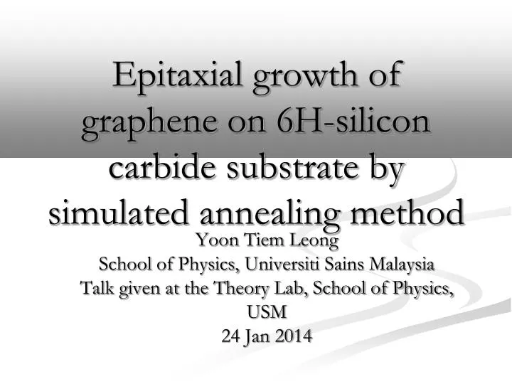
Yoon Tiem Leong School of Physics, Universiti Sains Malaysia Talk given at the Theory Lab, School of Physics, USM 24 Jan 2014. Epitaxial growth of graphene on 6H-silicon carbide substrate by simulated annealing method.

E N D
Yoon TiemLeong School of Physics, UniversitiSainsMalaysia Talk given at the Theory Lab, School of Physics, USM 24 Jan 2014 Epitaxial growth of graphene on 6H-silicon carbide substrate by simulated annealing method
We grew grapheneepitaxially on 6H-SiC(0001) substrate by the simulated annealing method. The mechanisms that govern the growth process were investigated by testing two empirical potentials, namely, the widely used Tersoff potential and its more refined version published years later by Erhart and Albe (TEA potential). We evaluated the reasonableness of our layers of graphene by calculating carbon-carbon (i) average bond-length, (ii) binding energy. The annealing temperature at which the graphene structure just coming into view at approximately 1200 K is unambiguously predicted by TEA potential and close to the experimentally observed pit formation at 1298 K. Abstract
How we construct the unit cell and supercell for 6H-SiC substrate • We refer • http://cst-www.nrl.navy.mil/lattice/struk/6h.html • to construct our 6H-SiC substrate.
The snapshots from the above webpage Figure 1: Snapshot from http://cst-www.nrl.navy.mil/lattice/struk/6h.html. The 6H-SiC belongs to the hexagonal class. For crystal in such a class, the lattice parameters and the angles between these lattice parameters are such that a = b ¹ c ; a = b = 90 degree, g= 120 degree.
Figure 2: Snapshot from http://cst-www.nrl.navy.mil/lattice/struk.xmol/6h.pos
Structure of the unit cell • Each unit cell of the 6H-SiC has a total of 12 basis atoms, 6 of them carbon, and 6 silicon. • Figure 2 displays: • (1) The coordinates of these atoms (listed in the last 12 rows in Figure 2). We note that only the Cartesian coordinates are to be used when preparing the input data for LAMMPS. • (2) Primitive vectors a(1), a(2), a(3) in the {X, Y, Z} basis (i.e. Cartesian coordinate system).
Procedure to construct rhombus-shaped 6H-SiC substrate • First, we determine the lattice constants, a , b (= a), c : • From Figure 2, the primitive vectors, a(1), a(2), a(3) are given respectively (in unit of nanometer) as • a(1) = (1.54035000, -2.66796446, 0 .00000000) • a(2) = (1.54035000, 2.66796446, 0.00000000) • a(3) = (.00000000, .00000000, 15.11740000). • Squaring a(1) and adding it to a(2) squared, we could easily obtain the value for the lattice parameter a, which is also equal to b by definition of the crystallographic group.
Lattice parameters • The lattice constants, as obtained from the above calculation, are a = 3.08 nm, b=3.08 nm, c = 15.11 nm. • Since the 6H-SiC belongs to a hexagonal class, = = 90 degree, = 120 degree.
Translation of lattice parameters into LAMMPS-readable unit • We refer to the instruction manual from the LAMMPS website in order to feed in the information of the lattice parameters into LAMMPS: • http://lammps.sandia.gov/doc/Section_howto.html#howto_12, section 6.12, Triclinic (non-orthogonal) simulation boxes • In LAMMPS, the units used are {lx, ly, lz; xy, xz, yz}. We need to convert {a, b, c; } into these units. This could be done quite trivially, via the conversion show in the right:
Raw unit cell of 6H-SiC • Based on the procedures described in previous slides, we constructed a LAMMPS data file for a raw 6H-SiC unit cell. • It represents a unit cell of 6H-SiC comprises of six hexagonal layers repeating periodically in the z-direction. • The resultant data file, named dataraw.xyz, is include in Figure 4. It is to be viewed using xcrysdens or VMD.
Figure 4 Sublayer of Si and C Sublayer of Si and C Sublayer of Si and C Sublayer of Si and C Sublayer of Si and C Figure 4: Visualization of the original unit cell’s atomic configuration as specified in dataraw.xyz. The coordinates of the atoms are also shown. There is a total of 12 atoms in the unit cell.
Raw unit cell of 6H-SiC • Each hexagonal layer consists of two sublayers. Each of these sublayers is comprised of Carbon and Silicon atoms (see Figure 4). • Note that the topmost atom is a Carbon. This means the (0001) surface of the 6H-SiC is Carbon terminated. • There is a total of 12 atoms it the original unit cell.
Modification for carbon-rich layer • Next, we shall modify the unit cell dataraw.xyz via the following procedure: • The Si atom (No. 9) is removed. The atom C (No. 5) is now translated along the z–direction to take up the z-coordinate left vacant by the removed Si atom (while the x- and y-coordinate remains unchanged).
Simulation method of graphene growth (one layer) • Simulated Annealing • Timestep = 0.5 fs • Increase the temperature slowly until it attains 300 Katapproximately 5˟1013K/s. • Equilibrating the system at 300 K for 20000 MD steps. • Raise the temperature of the system slowly to the desired T atapproximately 1013K/s. • Equilibrating the system at T for 30000 MD steps. • Cool down the system until 0.1 Kat 5x10¹²K/s • Extracting the result. 2.52 Å < 1 Å = 0.63 Å 2.0 Å Conjugate gradient minimization Simulated annealing
11 Atoms C 0.00000000 0.00000000 1.89572196 C0.00000000 0.00000000 9.45442196 Si 0.00000000 0.00000000 0.00000000 Si 0.00000000 0.00000000 7.55870000 C 1.54035000 0.88932149 10.07877058 C 1.54035000 -0.88932149 4.41276906 C 1.54035000 0.88932149 6.92981616 C 1.54035000 -0.88932149 -0.62888384 Si 1.54035000 -0.88932149 2.52007058 Si 1.54035000 0.88932149 5.03711768 Si 1.54035000 -0.88932149 -2.52158232 Figure 5: The content of data.singlelayer.xyz, detailing the coordinates of the atoms in a carbon-rich SiC substrate unit cell. Note that now only 11 atoms remain as one Si atom (atom 5). Content of data.singlelayer.xyz • The content of dataraw.xyz is now modified and renamed as data.singlelayer.xyz, which content is shown in Figure 5, and visualised in Figure 6.
Figure 6. : Visualization of the unit cell’s atomic configuration as specified in data.singlelayer.xyz. This is the carbon-rich substrate to be used for single layer graphene growth. Figure 6: carbon-rich unit cell of SiC 11 atoms per unit cell left as one Si atom (No. 9) has been removed.
Generating supercell • We then generated a supercell comprised of 12 x 12 x 1 unit cells as specified in data.singlelayer.xyz. • This is accomplished by using the command • replicate 12 12 1
Periodic BC • Periodic boundary condition is applied along the x-, y- and z-directions via the command: • boundary p p p • We created a vacuum of thickness 10 nm (along the z-direction) above and below the substrate. • The 12 x 12 x 1 supercell constructed according to the above procedure is visialised in Figure 7.
Figure 7 (a) Figure 7: A 1584-atom supercell mimicking a carbon-rich SiC substrate. It is made up of 12 x 12 x 1 unit cells as depicted in Figure 6. 7(a) Top view, 7(b) side view and 7(c) a tilted perspective are presented. Yellow: Carbon; Blue: Silicon.
Visualisation of the 12 x 12 x 1 supercell • There is a total of 1584 atoms in the simulation box. • Coordinates of all the atoms in the supercell can be obtained from LAMMPS’s trajectory file during the annealing process. • These coordinates are simply the atomic coordinates of the first step output during the MD run. • View the structure file 10101.xyz using VMD. • The 12 x 12 x 1 unit cell mimicking a Carbon-rich substrate will be used as our input structure to LAMMPS to simulate epitaxial graphene growth.
Monitor output here Figure 8. Annealing procedure based on suggestion by Prof. S.K. Lai. Annealing procedure • Once the data file for the Carbon-rich SiC substrate is prepared, we proceed to the next step to growth a single layer graphene via the process described in Figure 8 below. 1K 1 5 x 10¹³ K/s 5000 5000 steps
Implementation • To implement the above procedure, a fixed value of target annealing temperature was first chosen, e.g. Tanneal = 900 K. • We ran the LAMMPS input script (in.anneal) using a (fixed) target Tanneal. • We monitor the LAMMPS output while the system undergoes equilibration at the target annealing temperature (after the temperature has been ramped up gradually from 1 K).
Figure 9Temperature profile • A typical temperature profile that specifies how the temperature of the system being simulated changes as a function of step is illustrated, with the target temperature at Tanneal = 1200 K). Figure 9
Implementation (cont.) • If graphene is formed at a given target annealing temperature, the following phenomena during equilibrium (at that annealing temperature) will be observed: • (i) An abrupt formation of hexagonal rings by the carbon rich layer (visualize the lammps trajectory file using VMD in video mode), • (ii) an abrupt drop of biding energy, • (iii) an abrupt change of pressure. • In actual running of the LAMMPS calculation, we repeat the above procedure for a set of selected target annealing temperature one-by-one, Tanneal = 400 K, 500K, 1100K, 1200 K …, 2000 K.
Numerical parameters • The essential parameters used in annealing the substrate for single layered graphene growth: • 1. damping coefficient: 0.005 • 2. Timestep: 0.5 fs. • 3. Heating rate from 300 K -> target temperatures, 5 x 10¹³ K/s. • 4. Cooling rate: From target temperatures -> 1 K, 1 x 10¹³ K/s. • 5. Target temperatures: 700 K, 800 K, …, 2000 K. • 6. Steps for equilibration: (i) At 1K, 5000 steps. (ii) At 300 K, 20,000 steps, (iii) target annealing temp -> target annealing temp, 60,000 steps. • Essentially, all the parameters used are the same as that used by the NCU group.
Force fields • For single layer graphene formation, two force fields are employed: TEA and Tersoff. • As it turns out later, TEA shows a better results than Tersoff. We shall compare their results later.
0.63Å 0.22Å 1.89Å 1.99Å 0.624 Å 0.2276 Å 1.896 Å 1.9948 Å After minimization but before simulated annealing Configuration of the carbon-rich substrate before and after equilibration at T = 1.0 K for single-layered graphene formation Before minimisation After minimisation As comparison, this figure shows the geometry obtained by the NTCU group before and after minimisation
Formation of single layered graphene with thickness z=1 substrate, with TEA at 1200 K • http://www.youtube.com/watch?v=klkg2Rlf7Gk • Agrees with what Hannon and Tromp measured:
Data and results for single layer graphene formation • In the following slides, the following quantities are shown: • (i) Temperature vs. step (tempvsstep.dat) • (ii) Binding energy versus step during equilibration at target annealing temperature (bindingenergyvsstep.dat). • (iii) Average nearest neighbour (“bond length”) of the topmost carbon atoms versus step during equilibration at target annealing temperature (avenn_vs_step.dat). • (iv) Average distance between the topmost carbon atoms (cr3) and the Si atom (Si4) lying just below these carbon atoms vs step (distance34vsstep.dat). This is the distance between the graphene and the substrate just below it.
Definition of d34 for single layer graphene formation Top carbon-rich layer, (labeled as cr3) d34 = average distance between the carbon-rich layer and the substrate just below it Si atoms (labeled as Si4) SiC substrate
Figure 10(i): Tanneal = 1100 K. No graphene formed
Figure 10(ii): Tanneal = 1200 K. Graphene is formed
Determination of binding energy (BE) at a fixed Tanneal • Should an abrupt change in binding energy occurs at a given Tanneal during equilibration, such as that illustrated below (for Tanneal = 1200 K), how do we decide the value of the binding energy (which is step-dependent) for this annealing temperature? • We choose the value of the BE at the end of equilibration step, denoted as s. s is Tanneal-dependent: • s = 5000+85000+40*(temp-300) s s
BE vs. Tanneal • Based on the data shown in Figures 10, we abstract the value of BE at step = s from annealing temperature to plot the graph of BE vs Tanneal. • The values of BE (at step s) vs Tanneal is tabled in bdvstemp.dat. • The resultant curve is shown in Figure 11.
data\singlelayer\TEA\bdvstemp.dat Anneal temp binding energy 400 -5.880470833333334 500 -5.872215972222222 600 -5.8549182291666595 700 -5.853736979166666 800 -5.844029131944445 900 -5.8253253472222255 1000 1100 -5.810316180555554 1200 -6.647701284722221 1300 -6.830150555555552 1400 -6.844608055555553 1500 -6.713664999999995 1600 -6.833112638888893 1700 -6.747370833333332 1800 -6.877048993055555 1900 -6.709565694444447 Binding energy vs anneal temperature Figure 11
Average nearest neighbour (nn)(a.k.a ‘bond length’) vs anneal temperature • Based on the data shown in Figures 10, we abstract the value of average nn at step = s from each annealing temperature to plot the graph of ave nn vs Tanneal. • The resultant curve is shown in Figure 12.
Anneal temp average nn 400 1.750833424567148 500 1.746625140692055 600 1.7589214030309763 1.7419868390032442 800 1.7414136922144865 900 1.7589380688936933 100 1.7417389709279334 110 1.7344180027393463 1200 1.5027327808093742 1300 1.4693218689432666 1400 1.4764060075537178 Average nearest neighbour (nn) vs anneal temperature Figure 12
Anneal temp average distance cr3-Si6 400 2.1048033680555562 500 2.1063726736111175 • 2.105993090277779 • 2.105879791666668 • 800 2.1031867708333323 • 900 2.1202562847222266 • 1000 2.1176251041666685 • 1100 2.124162604166675 • 1200 2.4697990625000052 • 1300 2.560621458333336 • 1400 2.54777364583333 • 1500 2.6178477083333327 • 1600 2.6055096527777843 • 1700 2.722710520833341 • 1800 2.8183415972222177 • 1900 2.6691606597222215 Average distance between cr1 and Si6 vs anneal temperature
Data and results for single layer graphene formation with TEA • From the data generated, we conclude that: • Graphene formation is observed only when Tanneal= Tf (transition temperature) = 1200 K or above for TEA potential.
Outcome from Tersoff • We have also simulated with Tersoff force field. • The outcome are summarised in the next slide.
Tersoff vs. TEA Tersoff TEA
TEA vs Tersoff • TEA results compared better with experiment than TERSOFF did • TEA fitting of the three body interactions among the Si-C atoms is more rigorous; whereas Tersoff’s three body interactions are fitted with lesser accuracy.
Figure 13 Prepare a two-layered carbon-rich substrate by further knocking off two layers of Si atom, and then shift the topmost carbon atom layers to form two carbon rich layers. Thickness of the substrate is z=1. Conjugate gradient minimization Simulated annealing Conjugate gradient minimization 50 14