Chapter 5. Joint Probability Distributions and Random Sample
1.02k likes | 1.51k Vues
Chapter 5. Joint Probability Distributions and Random Sample. Weiqi Luo ( 骆伟祺 ) School of Software Sun Yat-Sen University Email : weiqi.luo@yahoo.com Office : # A313. Chapter 5: Joint Probability Distributions and Random Sample. 5.1. Jointly Distributed Random Variables

Chapter 5. Joint Probability Distributions and Random Sample
E N D
Presentation Transcript
Chapter 5. Joint Probability Distributions and Random Sample Weiqi Luo (骆伟祺) School of Software Sun Yat-Sen University Email:weiqi.luo@yahoo.com Office:# A313
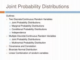
Chapter 5: Joint Probability Distributions and Random Sample • 5.1. Jointly Distributed Random Variables • 5.2. Expected Values, Covariance, and Correlation • 5. 3. Statistics and Their Distributions • 5.4. The Distribution of the Sample Mean • 5.5. The Distribution of a Linear Combination
5.1. Jointly Distributed Random Variables • The Joint Probability Mass Function for Two Discrete Random Variables Let X and Y be two discrete random variables defined on the sample space S of an experiment. The joint probability mass functionp(x,y) is defined for each pair of numbers (x,y) by
5.1. Jointly Distributed Random Variables • Let A be any set consisting of pairs of (x,y) values. Then the probability P[(X,Y)∈A] is obtained by summing the joint pmf over pairs in A: • Two requirements for a pmf
y p(x,y) 0 100 200 100 250 0.20 0.10 0.20 0.05 0.15 0.30 x 5.1. Jointly Distributed Random Variables • Example 5.1 A large insurance agency services a number of customers who have purchased both a homeowner’s policy and an automobile policy from the agency. For each type of policy, a deductible amount must be specified. For an automobile policy, the choices are $100 and $250, whereas for a homeowner’s policy the choices are 0, $100, and $200. Suppose an individual with both types of policy is selected at random from the agency’s files. Let X = the deductible amount on the auto policy, Y = the deductible amount on the homeowner’s policy Joint Probability Table
y p(x,y) 0 100 200 100 250 0.20 0.10 0.20 0.05 0.15 0.30 x 5.1. Jointly Distributed Random Variables • Example 5.1 (Cont’) p(100,100) =P(X=100 and Y=100) = 0.10 P(Y ≥ 100) = p(100,100) + p(250,100) + p(100,200) + p(250,200) = 0.75
5.1. Jointly Distributed Random Variables • The marginal probability mass function The marginal probability mass functions of X and Y, denoted by pX(x) and pY(y), respectively, are given by pY pX
y p(x,y) 0 100 200 100 250 0.20 0.10 0.20 0.05 0.15 0.30 x 5.1. Jointly Distributed Random Variables • Example 5.2 (Ex. 51. Cont’) The possible X values are x=100 and x=250, so computing row totals in the joint probability table yields px(100)=p(100,0 )+p(100,100)+p(100,200)=0.5 px(250)=p(250,0 )+p(250,100)+p(250,200)=0.5
y p(x,y) 0 100 200 100 250 0.20 0.10 0.20 0.05 0.15 0.30 x 5.1. Jointly Distributed Random Variables • Example 5.2 (Cont’) py(0)=p(100,0)+p(250,0)=0.2+0.05=0.25 py(100)=p(100,100)+p(250,100)=0.1+0.15=0.25 py(200)=p(100,200)+p(250,200)=0.2+0.3=0. 5 P(Y ≥ 100) = p(100,100) + p(250,100) + p(100,200) + p(250,200) = pY(100)+pY (200) =0.75
5.1. Jointly Distributed Random Variables • The Joint Probability Density Function for Two Continuous Random Variables Let X and Y be two continuous random variables. Then f(x,y) is the joint probability density functionfor X and Y if for any two-dimensional set A Two requirements for a joint pdf 1. f(x,y) ≥ 0; for all pairs (x,y) in R2 2.
5.1. Jointly Distributed Random Variables • In particular, if A is the two-dimensional rectangle {(x,y):a ≤ x ≤ b, c ≤ y ≤ d},then f(x,y) y Surface f(x,y) A = Shaded rectangle x
Verify that f(x,y) is a joint probability density function; • Determine the probability 5.1. Jointly Distributed Random Variables • Example 5.3 A bank operates both a drive-up facility and a walk-up window. On a randomly selected day, let X = the proportion of time that the drive-up facility is in use, Y = the proportion of time that the walk-up window is in use. Let the joint pdf of (X,Y) be
5.1. Jointly Distributed Random Variables • Marginal Probability density function The marginal probability density functionsof X and Y, denoted by fX(x) and fY(y), respectively, are given by Y Fixed y X Fixed x
5.1. Jointly Distributed Random Variables • Example 5.4 (Ex. 5.3 Cont’) The marginal pdf of X, which gives the probability distribution of busy time for the drive-up facility without reference to the walk-up window, is for x in (0,1); and 0 for otherwise. Then
5.1. Jointly Distributed Random Variables • Example 5.5 A nut company markets cans of deluxe mixed nuts containing almonds, cashews, and peanuts. Suppose the net weight of each can is exactly 1 lb, but the weight contribution of each type of nut is random. Because the three weights sum to 1, a joint probability model for any two gives all necessary information about the weight of the third type. Let X = the weight of almonds in a selected can and Y = the weight of cashews. The joint pdf for (X,Y) is
5.1. Jointly Distributed Random Variables • Example 5.5 (Cont’) 1: f(x,y) ≥ 0 (0,1) (x,1-x) (1, 0) x
5.1. Jointly Distributed Random Variables • Example 5.5 (Cont’) Let the two type of nuts together make up at most 50% of the can, then A={(x,y); 0≤x ≤1; 0 ≤ y ≤ 1, x+y ≤ 0.5} (0,1) x+y=0.5 (1, 0)
5.1. Jointly Distributed Random Variables • Example 5.5 (Cont’) The marginal pdf for almonds is obtained by holding X fixed at x and integrating f(x,y) along the vertical line through x: (0,1) (x,1-x) (1, 0) x
when X and Y are discrete when X and Y are continuous 5.1. Jointly Distributed Random Variables • Independent Random Variables Two random variables X and Y are said to be independent if for every pair of x and y values, Otherwise, X and Y are said to be dependent. Namely, two variables are independent if their joint pmf or pdf is the product of the two marginal pmf’s or pdf’s.
y p(x,y) 0 100 200 100 250 0.20 0.10 0.20 0.05 0.15 0.30 x 5.1. Jointly Distributed Random Variables • Example 5.6 In the insurance situation of Example 5.1 and 5.2 So, X and Y are not independent.
5.1. Jointly Distributed Random Variables • Example 5.7 (Ex. 5.5 Cont’) Because f(x,y) has the form of a product, X and Y would appear to be independent. However, although By symmetry
5.1. Jointly Distributed Random Variables • Example 5.8 Suppose that the lifetimes of two components are independent of one another and that the first lifetime, X1, has an exponential distribution with parameter λ1 whereas the second, X2, has an exponential distribution with parameter λ2. Then the joint pdf is Let λ1 =1/1000 and λ2=1/1200. So that the expected lifetimes are 1000 and 1200 hours, respectively. The probability that both component lifetimes are at least 1500 hours is
5.1. Jointly Distributed Random Variables • More than Two Random Variables If X1, X2, …, Xn are all discrete rv’s, the joint pmf of the variables is the function If the variables are continuous, the joint pdf of X1, X2, …, Xn is the function f(x1, x2, …, xn) such that for any n intervals [a1, b1], …, [an, bn], p(x1, x2, …, xn) = P(X1 = x1, X2 = x2, …, Xn = xn)
5.1. Jointly Distributed Random Variables • Independent The random variables X1, X2, …Xn are said to be independent if for every subset Xi1, Xi2,…, Xik of the variable, the joint pmd or pdf of the subset is equal to the product of the marginal pmf’s or pdf’s.
5.1. Jointly Distributed Random Variables • Multinomial Experiment An experiment consisting of n independent and identical trials, in which each trial can result in any one of r possible outcomes. Let pi=P(Outcome i on any particular trial), and define random variables by Xi=the number of trials resulting in outcome i (i=1,…,r). The joint pmf of X1,…,Xr is called the multinomial distribution. Note: the case r=2 gives the binomial distribution.
5.1. Jointly Distributed Random Variables • Example 5.9 If the allele of each of then independently obtained pea sections id determined and p1=P(AA), p2=P(Aa), p3=P(aa), X1= number of AA’s, X2=number of Aa’s and X3=number of aa’s, then If p1=p3=0.25, p2=0.5, then
5.1. Jointly Distributed Random Variables • Example 5.10 When a certain method is used to collect a fixed volume of rock samples in a region, there are four resulting rock types. Let X1, X2, and X3 denote the proportion by volume of rock types 1, 2 and 3 in a randomly selected sample. If the joint pdf of X1,X2 and X3 is k=144.
5.1. Jointly Distributed Random Variables • Example 5.11 If X1, …,Xn represent the lifetime of n components, the components operate independently of one another, and each lifetime is exponentially distributed with parameter, then
5.1. Jointly Distributed Random Variables • Example 5.11 (Cont’) If there n components constitute a system that will fail as soon as a single component fails, then the probability that the system lasts past time is therefore,
5.1. Jointly Distributed Random Variables • Conditional Distribution Let X and Y be two continuous rv’s with joint pdf f(x,y) and marginal X pdf fX(x). Then for any X values x for which fX(x)>0, the conditional probability density function of Y given that X=x is If X and Y are discrete, then is the conditional probability mass function of Y when X=x.
5.1. Jointly Distributed Random Variables • Example 5.12 (Ex.5.3 Cont’) X= the proportion of time that a bank’s drive-up facility is busy and Y=the analogous proportion for the walk-up window. The conditional pdf of Y given that X=0.8 is The probability that the walk-up facility is busy at most half the time given that X=0.8 is then
5.1. Jointly Distributed Random Variables • Homework Ex. 9, Ex.12, Ex.18, Ex.19
5.2 Expected Values, Covariance, and Correlation • The Expected Value of a function h(x,y) Let X and Y be jointly distribution rv’s with pmf p(x,y) or pdf f(x,y) according to whether the variables are discrete or continuous. Then the expected value of a function h(X,Y), denoted by E[h(X,Y)] or μh(X,Y) , is given by
5.2 Expected Values, Covariance, and Correlation • Example 5.13 Five friends have purchased tickets to a certain concert. If the tickets are for seats 1-5 in a particular row and the tickets are randomly distributed among the five, what is the expected number of seats separating any particular two of the five? The number of seats separating the two individuals is h(X,Y)=|X-Y|-1
5.2 Expected Values, Covariance, and Correlation • Example 5.13 (Cont’) x h(x,y) 1 2 3 4 5 1 -- 0 1 2 3 2 0 -- 0 1 2 3 1 0 -- 0 1 y 4 2 1 0 -- 0 5 3 2 1 0 --
5.2 Expected Values, Covariance, and Correlation • Example 5.14 In Example 5.5, the joint pdf of the amount X of almonds and amount Y of cashews in a 1-lb can of nuts was If 1 lb of almonds costs the company $1.00, 1 lb of cashews costs $1.50, and 1 lb of peanuts costs $0.50, then the total cost of the contents of a can is h(X,Y)=(1)X+(1.5)Y+(0.5)(1-X-Y)=0.5+0.5X+Y
5.2 Expected Values, Covariance, and Correlation • Example 5.14 (Cont’) The expected total cost is Note: The method of computing E[h(X1,…, Xn)], the expected value of a function h(X1, …, Xn) of n random variables is similar to that for two random variables.
5.2 Expected Values, Covariance, and Correlation • Covariance The Covariance between two rv’s X and Y is
5.2 Expected Values, Covariance, and Correlation • Illustrates the different possibilities. - - + - + + y y y μY μY μY - + - - + + x x x μX μX μX (a) positive covariance (b) negative covariance; (c) covariance near zero Here: P(x, y) =1/10
x 100 250 pX(x) .5 .5 5.2 Expected Values, Covariance, and Correlation • Example 5.15 The joint and marginal pmf’s for X = automobile policy deductible amount and Y = homeowner policy deductible amount in Example 5.1 were y y p(x,y) 200 0 100 100 0 250 .20 .10 .20 100 x pY(y) .25 .25 .5 250 .05 .15 .30 From which μX=∑xpX(x)=175 and μY=125. Therefore
5.2 Expected Values, Covariance, and Correlation • Proposition Note: • Example 5.16 (Ex. 5.5 Cont’) The joint and marginal pdf’s of X = amount of almonds and Y = amount of cashews were
5.2 Expected Values, Covariance, and Correlation • Example 5.16 (Cont’) fY(y) can be obtained through replacing x by y in fX(x). It is easily verified that μX= μY= 2/5, and Thus Cov(X,Y) = 2/15 - (2/5)2 = 2/15 - 4/25 = -2/75. A negative covariance is reasonable here because more almonds in the can implies fewer cashews.
5.2 Expected Values, Covariance, and Correlation • Correlation The correlation coefficient of X and Y, denoted by Corr(X,Y), ρX,Y or just ρ, is defined by • Example 5.17 It is easily verified that in the insurance problem of Example 5.15, σX= 75 and σY = 82.92. This gives The normalized version of Cov(X,Y) ρ = 1875/(75)(82.92)=0.301
5.2 Expected Values, Covariance, and Correlation • Proposition 1. If a and c are either both positive or both negative Corr(aX+b, cY+d) = Corr(X,Y) 2. For any two rv’s X and Y, -1 ≤ Corr(X,Y) ≤ 1. 3. If X and Y are independent, then ρ = 0, but ρ = 0 does not imply independence. 4. ρ = 1 or –1 iffY = aX+b for some numbers a and b with a ≠ 0.
5.2 Expected Values, Covariance, and Correlation • Example 5.18 Let X and Y be discrete rv’s with joint pmf It is evident from the figure that the value of X is completely determined by the value of Y and vice versa, so the two variables are completely dependent. However, by symmetry μX= μY= 0 and E(XY) = (-4)1/4 + (-4)1/4 + (4)1/4 + (4)1/4 = 0, so Cov(X,Y) = E(XY) - μX μY= 0 and thus ρXY= 0. Although there is perfect dependence, there is also complete absence of any linear relationship!
5.2 Expected Values, Covariance, and Correlation • Another Example X and Y are uniform distribution in an unit circle (1,0) Obviously, X and Y are dependent. However, we have
5.2 Expected Values, Covariance, and Correlation • Homework Ex. 24, Ex. 26, Ex. 33, Ex. 35
f(x) 0.05 x 0 15 5 10 5.3 Statistics and Their Distributions • Example 5.19 Given a Weibull Population with α=2, β=5 ~ μ= 4.4311, μ= 4.1628, δ=2.316 0.15 0.10
5.3 Statistics and Their Distributions • Example 5.19 (Cont’)
5.3 Statistics and Their Distributions • Example 5.19 (Cont’) Function of the sample observation A quantity #1 Sample 1 Function of the sample observation statistic A quantity #2 Population Sample 2 … Function of the sample observation A quantity #k Sample k