Download
1 / 21
210 likes | 335 Vues
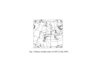
Fig. 1 Surface weather chart at 9 JST 21 July 1999. Observation. NARITA. 20mm/h- 10-20mm/h 1-10mm/h 1mm/h. HANEDA. 9JST 12JST 15JST 18JST 21JST.

E N D
Observation NARITA 20mm/h-10-20mm/h1-10mm/h1mm/h HANEDA 9JST 12JST 15JST 18JST 21JST Fig. 2 Hourly precipitation observed by operational radars of Japan Meteorological Agency from 9 JST to 21 JST on 21 July 1999. Precipitation was calibrated by the rain gages. Circles in the panel of 15 JST indicate the observation range of Narita and Haneda Doppler radars.
Fig. 3 Horizontal distribution of precipitation region (shaded region), surface temperature (solid line) and horizontal wind at 16 JST 21 July 1999. Barb and flag indicate the wind velocity of 2 m/s and 5 m/s, respectively.
Benchmark Case 10mm/h 5mm/h 1mm/h 9JST 12JST 15JST 18JST 21JST 10m/s Fig. 4 Precipitation region and horizontal wind at the height of 1.5km predicted from 9 JST 21 July 1999.
GEONET sitesDoppler radar sites NARITA HANEDA Fig.5 GEONET sites used to analyze PWV and SWV in the Kanto area (black squares). Two open circles indicate the positions of Doppler radar. Solid contour lines depict the topography with the interval of 500m.
GPS satellite Height GPS receiver Fig. 6 Schematic illustration of the calculation of SWV from the predicted density and specific humidity.
31.6 31.6 NARITA HANEDA 15.2 15.2 10.8 10.8 Layer 7.7 7.7 Height (km) Height (km) 4.9 4.9 Layer 2.7 2.7 1.1 1.1 0.3 0.3 Number of data Observed RW - first guess Observed RW - first guess (m/s) (m/s) Fig. 7 Distribution of the difference between the observed RW and the first guess.Vertical axes are the number and height of layers of MSM.
Number of data Observed vertical-scaled SWV - first guess value (mm) Fig. 8 Difference between the observed vertical-scaled SWV and the corresponding first guess value. Vertical axis indicates the number of data in each difference.
15.210.8 7.7 4.9 2.7 1.1 0.3 Layer Height (km) (m/s) Observation error of RW (m/s) Fig. 9 The observation error profile of the horizontal wind observed by the Satellite. Vertical axes indicate the number and height of layers of MSM.
RW&PWV Conventional data PWV Total Total Total 1 1 1 2 2 2 RW 1 PWV 2 PWV RW RW&SWV SWV Total Total 1 1 Total 1 2 2 2 1 1 RW RW 2 SWV 2 SWV Fig. 10 Variation of the cost function. Horizontal axes are the times of the iteration. Numbers in each panel indicated the times of analysis cycle.
RW EL=1.1 ° RW EL=1.1° PWV PWV - - - - + (a) Observation - (d) RW + + - - + + - - + + (b) First guess - (e) PWV - - + - - + - - - (c) Conventionaldata - + + + - (f) RW & PWV + - - + + - - Fig. 11 Radial wind at the elevation angle of 1.1 degree and precipitable water vapor at 15JST. Arrows and broken lines in RW fields indicate the horizontal wind inferred from RW data and the positions of RW=0. Squares with border of solid lines in PWV fields indicate PWV that are smaller than 58mm. From upper left to lower right panels are (a) observed fields, (b) first guess fields, (c) analyzed fields of 4d-Var DA of the conventional data (radiosonde etc), (d) analyzed fields of 4d-Var DA with RW added, (e) analyzed fields of 4d-Var DA with PWV added, and (f) analyzed fields of 4d-Var DA with RW and PWV added.
(c) Observation • (b) Conventional data (a) Benchmark 60mm/h-40-60mm/h20-40mm/h10-20mm/h1-10mm/h1mm/h 16JST FT=01 16JST mm/h mm/h mm/h mm/h 5m/s 5m/s 60mm/h-40-60mm/h20-40mm/h10-20mm/h1-10mm/h1mm/h 17JST 17JST FT=02 Fig. 12 Prediction of hourly precipitation and horizontal wind at 0.5 km from 15 JST, July 21, 1999. Upper row is 1 hour forecast (Valid time 16 JST) and lower row is 2 hour forecast (Valid time 17JST). From left to right columns are (a) the benchmark case, (b) prediction from 4d-Var DA of the conventional data, and (c) the hourly precipitation observed by JMA operational radars. Contour lines and shaded regions indicate hourly precipitation. Arrows in (a) and (b) are horizontal wind at 0.5 km. Large open arrows and the closed dotted ellipses indicate the major flows and the convergence zones.
(c) RW (b) SWV (a) PWV SWV FT=01 FT=01 FT=01 5mm/h 5mm/h 1mm/h 1mm/h FT=02 FT=02 FT=02 5m/s 5m/s Fig. 13 Same as Fig.12b, except for (a) prediction from 4d-Var DA with PWV added, (b) prediction from 4d-Var DA with SWV added, (c) prediction from 4d-Var DA with RW added.
(a) RW&PWV (b) RW&SWV FT=01 FT=01 5mm/h 1mm/h FT=02 FT=02 5m/s Fig. 14 Same as Fig. 12b but for (a) prediction from 4d-Var DA with RW and PWV added, (b) prediction from 4d-Var DA with RW and SWV added.
5mm/h 1mm/h 5m/s FT=05 FT=03 FT=06 Observation 60mm/h-40-60mm/h20-40mm/h10-20mm/h1-10mm/h1mm/h 18JST 19JST 20JST 21JST RW&PWV FT=04 Fig. 15 Prediction of hourly precipitation and horizontal wind at 0.5 km from 18 JST to 21 JST on 21 July 1999. Upper rows are the hourly precipitation observed by JMA radars. Lower rows are the predicted hourly precipitation from 3 hour forecast to 6 hour forecast (Valid time from 18 JST to 21 JST). Contour lines and shaded regions indicate hourly precipitation. Arrows are horizontal wind at 0.5 km. Large open arrows show major flows.
(b) Conventional data (b) Conventional data (c) RW (c) RW (c) -(b) (a) First guess (a) First guess - - B B - - - - - - - - - - - - + + - - + + + + + + 2019 2019 + + + + + + + + - - 1817 1817 - - - - - - 1615 1615 - - 1413 1413 - - - - 12 12 + + (d)-(b)(e)-(b)(e)-(c) + + [g/kg] [g/kg] - - - - - - - - 10m/s 10m/s A A - - + + + + + + - - - - 1.50 1.25 1.00 1.50 1.25 1.00 + + + + + + + + + + 0.75 0.50 0.25 0.75 0.50 0.25 Fig. 16 (a) Specific humidity and horizontal wind of first guess at the height of 0.5km. A line A-B is the position of the cross sections cross in Fig. 17. (b)-(e) are the differences of specific humidity and horizontal wind of the experiments of 'Conventional data', 'RW', 'PWV' and 'RW&PWV' from the first guess. Panels between (b)-(e) are the difference between both sides experiments. -0.25 -0.50 -0.75 -0.25 -0.50 -0.75 - - - - + + -1.00 -1.25 -1.50 [g/kg] -1.00 -1.25 -1.50 [g/kg] - - (d) PWV (e)-(d) (e) RW&PWV (e) RW&PWV - - + + - - - - + + - - - - + + + + + + + + + + + + - - - - - - 4m/s 4m/s
(d) RW&SWV-RW&PWV (c) RW&SWV (b) RW&PWV (a) First guess 18.0 16.5 15.0 1.50 1.25 1.00 500550600 500550600 500550600 500550600 ― + 0.75 0.50 0.25 13.5 12.0 10.5 + + + + 650700 650700 650700 650700 - - - Height (hPa) Height (hPa) Height (hPa) Height (hPa) - 9.0 7.5 6.0 -0.25 -0.50 -0.75 - 750800850 750800850 750800850 750800850 - - -1.00 -1.25 -1.50 [g/kg] 4.5 3.0 1.50 [g/kg] + + + - 900950 900950 900950 900950 A B A + B A B + A B 10m/s 4m/s Fig. 17 (a) Vertical cross section of specific humidity and horizontal wind of first guess along the line A-B in Fig. 16. (b) and (c) are the difference of specific humidity and horizontal wind of the experiments of ‘RW&PWV’ and ‘RW&SWV’ from the first guess. (d) is the difference between ‘RW&SWV’ and ‘RW&PWV’. Vertical axes in (a)-(d) are the pressure from 1000 hPa to 500 hPa.
(a) RW10&PWV (b) RW35&PWV FT=01 FT=01 FT=01 FT=01 5mm/h 1mm/h FT=02 FT=02 FT=02 FT=02 5m/s (c) HANEDA (d)NARITA Fig. 18 Same as Fig.12b, except for the prediction from 4d-Var DA with RW and PWV data added. Range of input RW data are (a) from surface to 1.0 km observed by Haneda and Narita radars, (b) from surface to 3.5km observed by Haneda and Narita radars, (c) from surface to 6.5 km observed by Haneda radar and (d) from surface to 6.5 km observed by Narita radar, respectively.
Radar_AMeDAS NARITA 20mm/h-10-20mm/h1-10mm/h1mm/h HANEDA 9JST 12JST 15JST 18JST 21JST Fig. 2 Hourly precipitation observed by operational radars of JMA from 9JST to 21JST on 21 July 1999. Precipitation was calibrated by the rain gages. Circles in the panel of 15JST indicate the observation range of Narita and Haneda Doppler radars. Radar_AMeDAS NARITA 10mm/h-1-10mm/h1mm/h HANEDA 9JST 12JST 15JST 18JST 21JST Fig. 2 Hourly precipitation observed by operational radars of JMA from 9JST to 21JST on 21 July 1999. Precipitation was calibrated by the rain gages. Circles in the panel of 15JST indicate the observation range of Narita and Haneda Doppler radars.
(d) RW&SWV-RW&PWV (c) RW&SWV (b) RW&PWV (a) First guess ― + + + + + - - - - - - - + + + - A B + B A B + A B 10m/s 4m/s Fig. 17 (a) Vertical cross section of specific humidity and horizontal wind of first guess along the line A-B in Fig16. (b) and (c) are the difference of specific humidity and horizontal wind of the experiments of ‘RW&PWV’ and ‘RW&SWV’ from the first guess. (d) is the difference between ‘RW&SWV’ and ‘RW&PWV’. Vertical axes in (a)-(d) are the pressure from 1000hPa to 500hPa.