Time Series Analysis of Particles and Fields data
190 likes | 335 Vues
This document explores advanced time series analysis methods applied to plasma and magnetic field characteristics at the magnetopause and magnetotail. Focused on the finite gyroradius effects, the analysis is pivotal in remotely sensing boundary speeds and thicknesses, enhancing our understanding of plasma dynamics in these regions. The findings highlight the importance of boundary conditions, particle gyroradii, and the implications for wave propagation and magnetospheric behavior, providing key insights for space weather prediction and plasma physics research.

Time Series Analysis of Particles and Fields data
E N D
Presentation Transcript
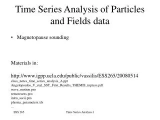
Time Series Analysis of Particles and Fields data • Magnetopause sounding Materials in: http://www.igpp.ucla.edu/public/vassilis/ESS265/20080514 class_notes_time_series_analysis_A.ppt Angelopoulos_V_etal_SST_First_Results_THEMIS_inpress.pdf wave_motion.pro remotesens.pro intro_ascii.pro plasma_parameters.xls … Time Series Analysis1
Finite gyroradius effects To Tail • Ion Gyroradius large compared to magnetospheric boundaries • Can be used to remotely sense speedand thickness of boundaries • Assumption is that boundary is sharpand flux has step function across • Application at the magnetopause • Application at the magnetotail • Can also be applied to waves ifparticle gradient is sufficiently high • Application on ULF waves atinner magnetosphere THEMIS To Earth To Sun Method exploits finite iongyroradius to remotely senseapproaching ion boundary and measure boundary speed (V⊥) Time Series Analysis2
At the magnetotail ri,thermal-tail (4keV,20nT)= ~325km ri,super-thermal (50keV,20nT)= ~2200km Plasma Sheet Thickness ~ 1-3 RE Boundary Layer Thickness ~500-2000km Current layer Thickness ~ 500-2000km Waves Across Boundary: ~1000-10,000km Along Boundary: ~Normal : 1-10 RE For magnetotail particles, the current layer and plasma sheet boundary layer are sharp compared to the superthermal ion gyroradius and the magnetic field is the same direction in the plasma sheet and outside (the lobe). This means we can use the measured field to determine gyrocenters both at the outer plasma sheet and the lobe, on either side of the hot magnetotail boundary. Time Series Analysis3
52o Side View (elevations) 25o SST: Elevationdirection (qDSL) SpinAxis -25o To Sun -52o ESA: Elevationdirection (qDSL) 33.75o 11.25o Time Series Analysis4
Top View (sectors) For ESA and SST (0=Sun) Spin axis To Sun (0o) 11.25o 33.75o Spin motiondirection ( fDSL) Normal to Sun, +90o Time Series Analysis5
B fieldazimuth (solid white) You care to time this!(+/- 90o to Bfield azimuth) Particle motion direction Coordinate: ( fDSL) Energy: 125-175keV Note: direction dependson spin axis. -B fieldazimuth (dashed white) Time Series Analysis6
Multiple spacecraft, energies, elevations A B …. D E Elev: 25deg E=30-50keV Elev: 25deg, E=80-120keV Time Series Analysis7
Vi_const 310km/sec/keV fci_cons 0.0152Hz/nT B 30nT Ti 40keV rho_ion 683km Ti 100keV rho_ion 1081km Ti 150keV rho_ion 1323km Ti 300keV rho_ion 1872km SC E (keV) detectord (deg) r time B 40 SPW -128.0 683.4 11:19:29 B 40 SPE -52.0 683.4 11:19:39 B 40 SEW -155.0 683.4 11:19:18 B 40 SEE -25.0 683.4 11:19:42 B 40 NPW 128.0 683.4 11:19:29 B 40 NPE 52.0 683.4 11:19:38 B 40 NEW 155.0 683.4 11:19:24 B 40 NEE 25.0 683.4 11:19:43 B 100 SPW -128.0 1080.5 11:19:17 B 100 SPE -52.0 1080.5 11:19:42 B 100 SEW -155.0 1080.5 11:19:20 B 100 SEE -25.0 1080.5 11:19:45 B 100 NPW 128.0 1080.5 11:19:20 B 100 NPE 52.0 1080.5 11:19:45 B 100 NEW 155.0 1080.5 11:19:23 B 100 NEE 25.0 1080.5 11:19:48 B 150 SPW -128.0 1323.4 11:19:10 B 150 SPE -52.0 1323.4 11:19:44 B 150 SEW -155.0 1323.4 11:19:14 B 150 SEE -25.0 1323.4 11:19:51 B 150 NPW 128.0 1323.4 11:19:23 B 150 NPE 52.0 1323.4 11:19:45 B 150 NEW 155.0 1323.4 11:19:13 B 150 NEE 25.0 1323.4 11:19:48 B 300 SPW -128.0 1871.5 11:19:10 B 300 SPE -52.0 1871.5 11:19:44 B 300 SEW -155.0 1871.5 11:19:14 B 300 SEE -25.0 1871.5 11:19:51 B 300 NPW 128.0 1871.5 11:19:23 B 300 NPE 52.0 1871.5 11:19:45 B 300 NEW 155.0 1871.5 11:19:13 B 300 NEE 25.0 1871.5 11:19:48 Note: NEE= North-Equatorial, East NPW=North-Equatorial, West Angles measured from East direction -25deg elevation, 90deg East = SEE +52deg elevation, 90deg East = NPE … Spin axis NPW NPE NEW NEE B SEW SEE SPW SPE Boundary Time Series Analysis8
Spin axis NPW NPE B V: NEE Part. direction NEW NEE SC d Y SEW SEE d r Z SPW SPE n Cold/tenuous plasma Y GCNEE n Hot/dense plasma e d Y Show: d=r*sin(d-e) Note: d negative if moving towards spacecraft Boundary Time Series Analysis9
Procedure • For a given e, determine variance of data for all d • Find minimum in variance, this determines e (boundary direction) • Speed distance as function of time determines boundary speed • intro_ascii,'remote_sense_A.txt',delta,rho,hh,mm,ss,nskip=13,format="(25x,f6.1,f8.1,3(1x,i2))" • ; • angle=fltarr(73) • chisqrd=fltarr(73) • for ijk=0,72 do begin • epsilon=float(ijk*5) • get_d_vs_dt,epsilon,hh,mm,ss,rho,delta,dist,times • yfit=dist & yfit(*)=0. • chi2=dist & chi2(*)=0. • coeffs=svdfit(times,dist,2,yfit=yfit,chisq=chi2) • angle(ijk)=epsilon • chisqrd(ijk)=chi2 • endfor • ipos=indgen(30)+43 • chisqrd_min=min(chisqrd(ipos),imin) • plot,angle,chisqrd • print,angle(ipos(imin)),chisqrd(ipos(imin)) • ; • stop Time Series Analysis10
Z D Y B A V ~ 70km/s 1000 km • Procedure • Note two minima (identical solutions) • One for approaching boundary at V>0 • One for receding boundary at V<0 • Convention that d<0 if boundarymoves towards spacecraftallows us to pick one of the two(positive slope of d versus time) Time Series Analysis11
tcross V [km/s] e [deg] D 11:19:27.6 75 270 B 11:19:31.8 70 280 A 11:19:38.4 80 275 Table 1. Results of remote sensing analysis on the inner probes Timing of the arrivals of the other signatures at the inner three spacecraft Time Series Analysis12
At the magnetopause ri,sheath (0.5keV,10nT)= ~200km ri,m-sphere (10keV,10nT)= ~1000km Magnetopause Thickness ~ 6000km Current layer Thickness ~ 500km FTE scale, Normal 2 Boundary: ~6000km Along Boundary: ~Normal : 1-3 RE For leaking magnetospheric particles, the currentlayer is sharp compared to the ion gyroradius andthe magnetic field is the same direction in the sheath and the magnetopause outside the current layer. This means we can use the measured field outside themagnetopause to determine gyrocenters both at the magnetopause and the magnetosheath on either side of the hot magnetopause boundary. Time Series Analysis13
Magnetopause encounter on July 12, 2007 Magnetic field angle is 60deg below spin plane and +120deg in azimuth i.e., anti-Sunward and roughly tangent to the magnetopause. The particle velocities, centered at 52deg above the spin plane, have roughly 90o pitch angles, with gyro-centers that were on the Earthward side of the spacecraft. The energy spectra of the NP particles show clearly the arrival of the FTE ahead of its magnetic signature, remotely sensing its arrival due to the finite gyroradius effect of the energetic particles. DT=55s, r(i,100keV, 28nT) =1150km, V=40km/s Time Series Analysis14
At the near-Earth magnetosphere Time Series Analysis15
At the near-Earth magnetosphere Time Series Analysis16
At the near-Earth magnetosphere Remote sensing of wavesin ESA data, at the mostappropriate coordinate System, I.e, field alignedcoordinates. gyro=0o => Earthward particles timespan,'7 11 07/10',2,/hours & sc='a' thm_load_state,probe=sc,/get_supp thm_load_fit,probe=sc,data='fgs',coord='gsm',suff='_gsm' thm_load_mom,probe=sc ; L2: onboard processed moms thm_load_esa,probe=sc ; L2: gmoms, omni spectra tplot,'tha_fgs_gsm tha_pxxm_pot tha_pe?m_density tha_pe?r_en_eflux' ; trange=['07-11-07/11:00','07-11-07/11:30'] thm_part_getspec, probe=['a'], trange=trange, angle='gyro', $ pitch=[45,135], other_dim='mPhism', $ ; /normalize, $ data_type=['peir'], regrid=[32,16] tplot,'tha_peir_an_eflux_gyro tha_fgs_gsm tha_pxxm_pot tha_pe?m_density tha_pe?r_en_eflux' Time Series Analysis17
At the near-Earth magnetosphere Same as before but using keyword: /normalize I.e., anisotropy is normalized to 1, to ensure flux variations do not affect anisotropy calculation. trange=['07-11-07/11:00','07-11-07/11:30'] thm_part_getspec, probe=['a'], trange=trange, angle='gyro', $ pitch=[45,135], other_dim='mPhism', $ /normalize, $ data_type=['peir'], regrid=[32,16] tplot,'tha_peir_an_eflux_gyro tha_fgs_gsm tha_pxxm_pot tha_pe?m_density tha_pe?r_en_eflux' Time Series Analysis18
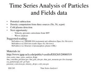
Topics for May 19 class • Potential subtraction • Cold plasma detection • Density computation from three sources (Ne, Ni, scpot) • Velocity, pressure corrections from SST • Waves analysis Time Series Analysis19