Efficient Stackelberg Routing Strategies for Network Congestion Optimization
290 likes | 315 Vues
Explore Stackelberg routing in algorithmic game theory, an approach where some players cooperate while others act selfishly, determining paths to lead to good Nash Equilibrium outcomes. Investigate Pigou's and Braess's networks, comparing optimal and Nash flows. Consider Price of Anarchy and strategies for minimum latency. Analyze LLF Strategy for assigning cooperative players to optimal paths to minimize congestion in network flow. Delve into complexities of finding the best strategy in NP-hard problems.

Efficient Stackelberg Routing Strategies for Network Congestion Optimization
E N D
Presentation Transcript
Stackelberg Strategies Algorithmic Game Theory Course Co.RE.Lab. - N.T.U.A. TexPoint fonts used in EMF. Read the TexPoint manual before you delete this box.: AAAAAAAA
Stackelberg Routing • In (classic) selfish routing all players act selfishly. • In Stackelberg routing there exist players willing to cooperate for social welfare (a fraction of the total players). • Both Selfish and Cooperative players are present. • Leader determines the paths of the coordinated players. • Selfish players (followers) minimize their own cost. • Nash Equilibria are considered as the possible outcomes of the game. • A Stackelberg Strategyis an algorithm that allocatespathstocoordinated players so as to lead selfish players to a good Nash Equilibrium.
Example: Pigou’s Network c(x)=x s t One unit of flow is to be routed from s to t c(x)=1
Example: Pigou’s Network c(x)=x Flow = ½ Optimal flow s t One unit of flow is to be routed from s to t c(x)=1 Flow = ½
Example: Pigou’s Network c(x)=x Flow = ½ Optimal flow s t One unit of flow is to be routed from s to t c(x)=1 Flow = ½ (Classic) Nash flow x Flow = 1 s t 1
Example: Pigou’s Network c(x)=x Flow = ½ Optimal flow s t One unit of flow is to be routed from s to t c(x)=1 Flow = ½ Nash flow when a fraction αof (coordinated) playersis sent through the lower edge (Classic) Nash flow x x Flow = 1 Flow = 1-α s t s t 1 1 Flow = α
Example: Braess’s Network x 1 One unit of flow is to be routed from s to t 0 s t x 1
Example: Braess’s Network ½ ½ x 1 One unit of flow is to be routed from s to t 0 s t ½ ½ x 1 Optimal flow
Example: Braess’s Network ½ ½ x 1 One unit of flow is to be routed from s to t 0 s t ½ ½ x 1 Optimal flow (Classic) Nash flow 1 x 1 0 s t 1 1 x
Example: Braess’s Network ½ ½ x 1 One unit of flow is to be routed from s to t 0 s t ½ ½ x 1 Optimal flow Nash flow when a fraction αof coordinated playersis sent through the lower edge (Classic) Nash flow α/2 1 x 1 x 1 1-α 0 0 s t s t 1 1 1 x x α/2
Slightly more formal • We will consider single commodity networks. • An instance in such networks: • Assume that a fraction α of the players are cooperative. • A Stackelberg strategy assigns cooperative players to paths. • They induce a congestion • A new game is “created”: • Where
In the “new” game • Selfish players choose paths (as usual), and Nash flows are considered as the possible outcomes of the game (as usual). • On Equilibrium, selfish players induce a congestion • The Price of Anarchy is
The Central Questions • Given a Stackelberg routing instance, we can ask: • Among all Stackelberg strategies, can we characterize and/or compute the strategy inducing the Stackelberg equilibrium - i.e., the eq. of minimum total latency? • What is the worst-case ratio between the total latency of the Stackelberg eq. and that of the optimal assignment of users to paths?
Finding best strategy: NP-hard Reduction from problem: Given n positive integers is there an satisfying: Given an instance of create an instance of stackelberg routing: • A network G with n+1parallel links • Demand: • ¼ of the players are followers • Cost functions:
LLF Strategy • Largest Latency First (LLF): • Compute an optimal configuration • Assign coordinated players to optimal paths of largest latency
LLF Strategy • Largest Latency First (LLF): • Compute an optimal configuration • Assign coordinated players to optimal paths of largest latency 6 units to be routed. 4 x s t 2x
LLF Strategy • Largest Latency First (LLF): • Compute an optimal configuration • Assign coordinated players to optimal paths of largest latency 6 units to be routed. 4 Flow =3 x Opt routes: • 3 to upper edge • 2 to middle edge • 1 to lower edge Flow =2 s t 2x Flow = 1
LLF Strategy • Largest Latency First (LLF): • Compute an optimal configuration • Assign coordinated players to optimal paths of largest latency 6 units to be routed. 4 Flow =3 x Opt routes: • 3 to upper edge • 2 to middle edge • 1 to lower edge Flow =2 s t 2x Flow = 1 4 In Nash Flow players are routed: • 4 to middle edge • 2 to lower edge x s t Flow=4 2x Flow=2 Nash Flow
LLF Strategy • Largest Latency First (LLF): • Compute an optimal configuration • Assign coordinated players to optimal paths of largest latency 6 units to be routed. 4 Flow =3 x Opt routes: • 3 to upper edge • 2 to middle edge • 1 to lower edge Flow =2 s t 2x Flow = 1 4 In Nash Flow players are routed: • 4 to middle edge • 2 to lower edge x s t Flow=4 2x Flow=2 Nash Flow
LLF Strategy • Largest Latency First (LLF): • Compute an optimal configuration • Assign coordinated players to optimal paths of largest latency 6 units to be routed. 4 Flow =3 x Opt routes: • 3 to upper edge • 2 to middle edge • 1 to lower edge Flow =2 s t 2x Flow = 1
LLF Strategy • Largest Latency First (LLF): • Compute an optimal configuration • Assign coordinated players to optimal paths of largest latency 6 units to be routed. 4 Flow =3 x Opt routes: • 3 to upper edge • 2 to middle edge • 1 to lower edge Flow =2 s t 2x Flow = 1 4 Flow =1½ LLF controlling ¼ players, e.g. 1½ units, routes: • 1½ to upper edge x s t Flow=3 2x Flow=1½ Nash Flow
LLF Strategy • Largest Latency First (LLF): • Compute an optimal configuration • Assign coordinated players to optimal paths of largest latency 6 units to be routed. 4 Flow =3 x Opt routes: • 3 to upper edge • 2 to middle edge • 1 to lower edge Flow =2 s t 2x Flow = 1 4 Flow =1½ LLF controlling ¼ players, e.g. 1½ units, routes: • 1½ to upper edge x s t Flow=3 2x Flow=1½ Nash Flow
LLF Strategy • Largest Latency First (LLF): • Compute an optimal configuration • Assign coordinated players to optimal paths of largest latency 6 units to be routed. 4 Flow =3 x Opt routes: • 3 to upper edge • 2 to middle edge • 1 to lower edge Flow =2 s t 2x Flow = 1
LLF Strategy • Largest Latency First (LLF): • Compute an optimal configuration • Assign coordinated players to optimal paths of largest latency 6 units to be routed. 4 Flow =3 x Opt routes: • 3 to upper edge • 2 to middle edge • 1 to lower edge Flow =2 s t 2x Flow = 1 4 Flow =3 LLF controlling ½ players, e.g. 3 units, routes: • 3 to upper edge x s t Flow=2 2x Flow=1 Nash Flow
LLF Strategy • Largest Latency First (LLF): • Compute an optimal configuration • Assign coordinated players to optimal paths of largest latency 6 units to be routed. 4 Flow =3 x Opt routes: • 3 to upper edge • 2 to middle edge • 1 to lower edge Flow =2 s t 2x Flow = 1 4 Flow =3 LLF controlling ½ players, e.g. 3 units, routes: • 3 to upper edge x s t Flow=2 2x Flow=1 Nash Flow
LLF in parallel links Let α be the fraction of the cooperative players. Theorem 1: In parallel links LLF induces an assignment of cost no more than 1/α times the OPT: Proof by induction: When LLF saturates a link we can restrict to the instance that has: • this link deleted and • fraction of players the “remainders” of the previous instance. Some problems: • LLF may fail to saturate any link. No problem: Let m be the “heaviest” link. If L is the cost of selfish players and x* is the optimal assignment, it is • When a link gets saturated selfish users could use it. No problem: There is an induced equilibrium that doesn’t use it.
Networks with UnboundedPoA Theorem: Let and . There is an instance such that for any Stackelberg strategy inducing s, it is: Proof: The network is the following The demands are: (total flow=1) Cost functions: B=1, C=0 and A is
LLF in parallel links Let oe denote the optimal congestion Lemma: The proof follows from the variational inequality, similar to the “classic” result.
LLF in parallel links Let oe denote the optimal congestion Lemma: The proof follows from the variational inequality, similar to the “classic” result. Theorem 2: Proof: and . It is This is maximized for with maximum value