Linear Programming
Linear Programming. Simplex method - II. Objectives. Objectives To discuss the Big-M method Discussion on different types of LPP solutions in the context of Simplex method Discussion on maximization verses minimization problems. Big-M Method.

Linear Programming
E N D
Presentation Transcript
Linear Programming Simplex method - II Optimization Methods: M3L4
Objectives Objectives • To discuss the Big-M method • Discussion on different types of LPP solutions in the context of Simplex method • Discussion on maximization verses minimization problems Optimization Methods: M3L4
Big-M Method Simplex method forLP problem with ‘greater-than-equal-to’ ( ) and ‘equality’ (=) constraints needs a modified approach. This is known as Big-M method. • The LPP is transformed to its standard form by incorporating a large coefficient M Optimization Methods: M3L4
Transformation of LPP for Big-M method • One ‘artificial variable’ is added to each of the ‘greater-than-equal-to’ (≥) and equality (=) constraints to ensure an initial basic feasible solution. • Artificial variables are ‘penalized’ in the objective function by introducing a large negative (positive) coefficient for maximization (minimization) problem. • Cost coefficients, which are supposed to be placed in the Z-row in the initial simplex tableau, are transformed by ‘pivotal operation’ considering the column of artificial variable as ‘pivotal column’ and the row of the artificial variable as ‘pivotal row’. • If there are more than one artificial variables, step 3 is repeated for all the artificial variables one by one. Optimization Methods: M3L4
Example Consider the following problem Optimization Methods: M3L4
Example • After incorporating the artificial variables where x3 is surplus variable, x4 is slack variable and a1 and a2 are the artificial variables Optimization Methods: M3L4
Transformation of cost coefficients Considering the objective function and the first constraint Pivotal Row Pivotal Column the cost coefficients are modified as By the pivotal operation Optimization Methods: M3L4
Transformation of cost coefficients Considering the modified objective function and the third constraint Pivotal Row Pivotal Column the cost coefficients are modified as By the pivotal operation Optimization Methods: M3L4
Construction of Simplex Tableau Corresponding simplex tableau Pivotal row, pivotal column and pivotal elements are shown as earlier Optimization Methods: M3L4
Simplex Tableau…contd. Successive simplex tableaus are as follows: Optimization Methods: M3L4
Simplex Tableau…contd. Optimization Methods: M3L4
Simplex Tableau…contd. Optimality has reached. Optimal solution isZ = 36withx1 = 2andx2 = 6 Optimization Methods: M3L4
Simplex method: ‘Unbounded’, ‘Multiple’ and ‘Infeasible’ solutions Unbounded solution • If at any iteration no departing variable can be found corresponding to entering variable, the value of the objective function can be increased indefinitely, i.e., the solution is unbounded. Optimization Methods: M3L4
Simplex method: ‘Unbounded’, ‘Multiple’ and ‘Infeasible’ solutions Multiple (infinite) solutions • If in the final tableau, one of the non-basic variables has a coefficient 0 in the Z-row, it indicates that an alternative solution exists. • This non-basic variable can be incorporated in the basis to obtain another optimal solution. • Once two such optimal solutions are obtained, infinite number of optimal solutions can be obtained by taking a weighted sum of the two optimal solutions. Optimization Methods: M3L4
Simplex method: Example of Multiple (indefinite) solutions Consider the following problem • Only modification, compared to earlier problem, is that the coefficient of x2 is changed from 5 to 2 in the objective function. • Thus the slope of the objective function and that of third constraint are now same, which leads to multiple solutions Optimization Methods: M3L4
Simplex method: Example of Multiple (indefinite) solutions Following similar procedure as described earlier, final simplex tableau for the problem is as follows: Optimization Methods: M3L4
Simplex method: Example of Multiple (indefinite) solutions As there is no negative coefficient in the Z-row optimal solution is reached. Optimal solution isZ = 18withx1 = 6andx2 = 0 However, the coefficient of non-basic variable x2is zero in the Z-row Another solution is possible by incorporating x2 in the basis Based on the , x4 will be the exiting variable Optimization Methods: M3L4
Simplex method: Example of Multiple (indefinite) solutions If one more similar step is performed, previous simplex tableau will be obtained back So, another optimal solution isZ = 18withx1 = 2andx2 = 6 Optimization Methods: M3L4
Simplex method: Example of Multiple (indefinite) solutions Thus, two sets of solutions are: and Other optimal solutions will be obtained as where For example, let b = 0.4, corresponding solution is Note that values of the objective function are not changed for different sets of solution; for all the cases Z = 18. Optimization Methods: M3L4
Simplex method: ‘Unbounded’, ‘Multiple’ and ‘Infeasible’ solutions Infeasible solution • If in the final tableau, at least one of the artificial variables still exists in the basis, the solution is indefinite. Optimization Methods: M3L4
Minimization versus maximization problems • Simplex method is described based on the standard form of LP problems, i.e., objective function is of maximization type • However, if the objective function is of minimization type, simplex method may still be applied with a small modification Optimization Methods: M3L4
Minimization versus maximization problems The required modification can be done in either of following two ways. • The objective function is multiplied by -1 so as to keep the problem identical and ‘minimization’ problem becomes ‘maximization’. This is because minimizing a function is equivalent to the maximization of its negative • While selecting the entering nonbasic variable, the variable having the maximum coefficient among all the cost coefficients is to be entered. In such cases, optimal solution would be determined from the tableau having all the cost coefficients as non-positive ( ) Optimization Methods: M3L4
Minimization versus maximization problems • One difficulty, that remains in the minimization problem, is that it consists of the constraints with ‘greater-than-equal-to’ ( ) sign. For example, minimize the price (to compete in the market), however, the profit should cross a minimum threshold. Whenever the goal is to minimize some objective, lower bounded requirements play the leading role. Constraints with ‘greater-than-equal-to’ ( ) sign are obvious in practical situations. • To deal with the constraints with ‘greater-than-equal-to’ ( ) and equality sign, Big-M method is to be followed as explained earlier. Optimization Methods: M3L4
Thank You Optimization Methods: M3L4

