Introduction to Spectroscopy and Spectrographs
Learn about spectroscopy, spectral resolution, dispersion, and different types of spectrographs. Explore how light is split into spectral components using prisms, gratings, and more. Understand spatial info retrieval and spectral resolution limitations in spectroscopy.

Introduction to Spectroscopy and Spectrographs
E N D
Presentation Transcript
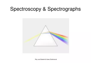
Spectroscopy & Spectrographs Roy van Boekel & Kees Dullemond
Overview • Spectrum, spectral resolution • Dispersion (prism, grating) • Spectrographs • longslit • echelle • fourier transform • Multiple Object Spectroscopy
Spectroscopy: what do we measure? • Spectrum = the intensity (or flux) of radiation as a function of wavelength • “Continuous” sampling in wavelength (as opposed to imaging, where we integrate over some finite wavelength range) • Note: In practice, when using CCDs for spectroscopy, one also integrates over finite wavelength ranges – they are just very narrow compared to the wavelength itself: Pixel width Δν << ν • Sampling is continuous but the spectral resolution is limited by the design of the spectrograph • Spectrum in classical sense holds no direct spatial information. Many spectrographs allow retrieving spatial info in 1 dimension, some even in 2 (“integral field units”)
Spectral resolution • Smallest separation in wavelength that can still be distinguished by instrument, usually given as fraction of and denoted by R: or alternatively useful, though somewhat arbitrary working definition
Basic spectrograph layout • a means to isolate light from the source in the focal plane, usually a slit • “collimator” to make parallel beams on the dispersive element • dispersive element, e.g. a prism or grating. Reflection gratings much more frequently used than transmission gratings • “Camera”: imaging lens to focus beams in the (detector) focal plane + detector to record the signal
Dispersion Splitting up light in its spectral components achieved by one of two ways: • differential refraction • prism • interference • reflection/transmission grating • fourier transform • (Farby-Perot) 6
Prism • general light path through prism: one can show that: • dispersion is maximum for a symmetrical light path • dispersion is maximum for grazing incidence. Corresponding top angle depends on refractive index of material. E.g. ~74° for heavy flint glass • However: most light is reflected instead of refracted for grazing incidence. In practice, smaller are used (60° and 30° are common choices)
Prism dispersion curve strongly non-linear, dispersion in blue much stronger than in red part of spectrum 8
Prism spectrograph layout 9 Credit: C.R. Kitchin “Astrophysical techniques” CRC Press, ISBN 13: 978-1-4200-8243-2
θ Young’s double slit experiment double slit lens screen incident wave d θ
Optical path difference: Phase difference: ΔP Add the two waves: Intensity is amplitude-squared: Young’s double slit experiment double slit lens screen incident wave d θ
Optical path difference: Phase difference: ΔP Add the three waves, and take the norm: Now a triple slit experiment... triple slit lens screen incident wave d θ
0th order 1st order 2nd order Adding more slits... N=16
Width of the peaks N=4 Peak width is therefore: For with one has (Later: Relevance for spectral resolution)
0th order 1st order 2nd order Now do 3 different wavelengths N=4 Green is here the reference wavelength λ. Blue/red is chosen such that its 1st order peak lies in green’s first null on the left/right of the 1st order.
0th order 1st order 2nd order Now do 3 different wavelengths N=8 Keeping 3 wavelengths fixed, but increasing N
0th order 1st order 2nd order Now do 3 different wavelengths N=16 Keeping 3 wavelengths fixed, but increasing N
0th order 1st order 2nd order Now do 3 different wavelengths N=4 Green is here the reference wavelength λ. Blue/red is chosen such that its 1st order peak lies in green’s first null on the left/right of the 1st order.
0th order 1st order 2nd order Spectral resolution: Now do 3 different wavelengths N=8 Green is here the reference wavelength λ. Blue/red is chosen such that its 1st order peak lies in green’s first null on the left/right of the 1st order.
0th order 1st order 2nd order Spectral resolution: Let’s look at the 2nd order N=8 Green is here the reference wavelength λ. Blue/red is chosen such that its 1st order peak lies in green’s first null on the left/right of the 1st order.
Let’s look at the 2nd order m=4 m=0 m=1 m=2 m=3 N=8 Green is here the reference wavelength λ. Blue/red is chosen such that its 1st order peak lies in green’s first null on the left/right of the 1st order.
Let’s look at the 2nd order m=2 N=8 Zoom-in around 2nd order Green is here the reference wavelength λ. Blue/red is chosen such that its 1st order peak lies in green’s first null on the left/right of the 1st order.
Let’s look at the 2nd order m=4 m=0 m=1 m=2 m=3 N=8 Green is here the reference wavelength λ. Blue/red is chosen such that its 1st order peak lies in green’s first null on the left/right of the 1st order.
Spectral resolution: Let’s look at the 2nd order m=4 m=0 m=1 m=2 m=3 N=8 Green is here the reference wavelength λ. Blue/red is chosen such that its 2nd order peak lies in green’s first null on the left/right of the 2nd order.
Let’s look at the 3rd order m=4 m=0 m=1 m=2 m=3 N=8 Green is here the reference wavelength λ. Blue/red is chosen such that its 3rd order peak lies in green’s first null on the left/right of the 3rd order. Spectral resolution:
General formula m=4 m=0 m=1 m=2 m=3 N=8 Green is here the reference wavelength λ. Blue/red is chosen such that its mth order peak lies in green’s first null on the left/right of the mth order. Spectral resolution:
Building a spectrograph from this Place a CCD chip here Make sure to have small enough pixel size to resolve the individual peaks.
Overlapping orders m=4 m=0 m=1 m=2 m=3 N=8 Going to higher orders means higher spectral resolution. But it also means: a smaller spectral range, because the “red” wavelengths of order m start overlapping with the “blue” wavelengths of order m+1
Effect of slit width triple slit lens screen incident wave d w
Effect of slit width single slit lens screen incident wave As we know from the chapter on diffraction: This gives the sinc function squared: w
Effect of slit width N=16 d/w=8
Grating • many parallel “slits” called “grooves” • Transmission gratings and reflection gratings • width of principal maximum (distance between peak and first zeros on either side): • “Blazing”: tilt groove surfaces to concentrate light towards certain direction controls in which order m light of given gets concentrated Credit: C.R. Kitchin “Astrophysical techniques” CRC Press, ISBN 13: 978-1-4200-8243-2 blazed reflection grating
blazed transmission grating Grating, spectral resolution • resolution in wavelength:
w -i d Reflection grating with groove width w and groove spacing d
Basic grating spectrograph layout 40 Credit: C.R. Kitchin “Astrophysical techniques” CRC Press, ISBN 13: 978-1-4200-8243-2
Basic grating spectrograph layout Note: The word “slit” is here meant with a different meaning: Not a dispersive element, but a method to isolate a source on the image plane for spectroscopy. From here onward, “slit” will have this meaning. Dispersive slit = groove on a grating. 41 Credit: C.R. Kitchin “Astrophysical techniques” CRC Press, ISBN 13: 978-1-4200-8243-2
Longslit spectrum • Very basic setup: entrance slit in focal plane, with dispersive element oriented parallel to slit (e.g. grooves of grating aligned with slit) • 1 spatial dimension (along slit) and 1 spectral dimension (perpendicular to slit) on the detector • Spectral resolution set by dispersive element, e.g. Nm for grating. • Spectrum can be regarded as infinite number of monochromatic images of entrance slit • projected width of entrance slit on detector must be smaller than projected size of resolution element on detector, e.g. for grating: where s is the physical slit width and 1 is the collimator focal length • slit width often expressed in arcseconds: where F is the effective focal length of the telescope beam entering the slit spatial direction
Example longslit spectrum spatial direction wavelength • high spectral resolution longslit spectrum of galaxy • Continuum emission from stars, several emission lines from star forming regions in galaxy
Gratings: characteristics • Light dispersed. If d ~ w most light goes into 1 or 2 orders at given . Light of (sufficiently) different gets mostly sent to different orders • Light from different orders may overlap (bad, need to deal with that!) • Spectral resolution scales with fringe order m and is nearly constant within a fringe order ~linear dispersion (in contrast to prism!) • Gratings are often tilted with respect to beam. Slightly different expression for positions of interference maxima: or equivalently i is the angle between the grating and the incoming beam. This expression is called the “grating equation”
long go into low m, short go into high m I m m m + i [deg] The “blaze function” describes the transmittance of light transmitted or reflected into each order. It is the “envelope” of the interference pattern (i.e. diffraction due to finite width of single groove, D)
m I m m Blaze function vs. wavelength
Order overlap in grating • Each order gives its own spectrum. These can overlap in the focal plane: at a given pixel on the detector we can get light from several orders (with different ) • We must reject light from the unwanted orders. Solution: • For low orders m (low spectral resolution, large free spectral range) one can use a filter that blocks light from the other orders • For high orders m (the free spectral range is very small), use “cross disperser”: a second dispersive element (usually a prism), mounted with the dispersion direction perpendicular to that of the grating. Causes different orders to be spatially offset on the chip. Advantage: multiple orders can be measured simultaneously. High spectral resolution and large coverage can be obtained simultaneously. “Echelle spectrograph”
Echelle grating • R m. For high spectral resolution, use high order. • Relatively large groove spacing (few grooves/mm) but very high blazing angle. Concentrate light in high orders. • Strong order overlap (solution: “cross-dispersion”, more later ...) Echelle grating Credit: C.R. Kitchin “Astrophysical techniques” CRC Press, ISBN 13: 978-1-4200-8243-2
CCD Echelle grating: cross dispersion m=103 m=102 m=101 m=100 m=99 m=98 m=97 m=96 Without cross dispersion: different wavelength ranges overlap. With cross dispersion: You get multiple short spectra. Note of caution: Above cartoon is not exact: colors should be sorted vertically; but it shows the principle of separating orders.
CCD Echelle grating: cross dispersion m=103 m=102 m=101 m=100 m=99 m=98 m=97 m=96 Strong blazing angle means that you focus the light on the part of the focal plane where the CCD is. Avoids waste of light.