Download

1 / 21
210 likes | 422 Vues
Logic Synthesis in IC Design and Associated Tools Binary Decision Diagrams. Wang Jiang Chau Grupo de Projeto de Sistemas Eletrônicos e Software Aplicado Laboratório de Microeletrônica – LME Depto. Sistemas Eletrônicos Universidade de São Paulo. Binary Decision Diagrams- 1.

E N D
Logic Synthesis in IC Design and Associated Tools Binary Decision Diagrams Wang Jiang Chau Grupo de Projeto de Sistemas Eletrônicos e Software Aplicado Laboratório de Microeletrônica – LME Depto. Sistemas Eletrônicos Universidade de São Paulo
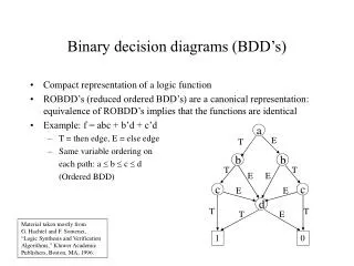
Binary Decision Diagrams- 1 • Binary decision diagrams (BDDs) can be represented by trees or rooted DAGs, where decisions are associated with vertices. • Ordered binary decision diagrams (OBDDs) assume an ordering on the decision variables. • Can be transformed into canonical forms, reduced ordered binary decision diagrams (ROBDDs) • Operations on ROBDDs can be made in polynomial time of their size i.e. vertex set cardinality
Binary Decision Diagrams- 2 • An OBDD is a rooted DAG with vertex set V. Each non-leaf vertex has as attributes • a pointer index(v) {1,2,…n} to an input variable {x1,x2,…,xi,…,xn} . • Two children low(v) and high(v) V. • A leaf vertex v has as an attribute a value value(v) B. • For any vertex pair {v,low(v)} (and {v,high(v)}) such that no vertex is a leaf, index(v)<index(low(v))(index(v)<index(high(v))
Binary Decision Diagrams- 3 • An OBDD with root v denotes a function fv such that • If v is a leaf with value(v)=1, then fv=1 • If v is a leaf with value(v)=0, then fv=0 • If v is not a leaf and index(v)=i, then fv= xi ’.f low(v) + xi.f high(v) f=(a+b).c For a,c,d odering and Shannon´s expansion f= (a+b).c= = a’.fa’+a.fa = a’.(cb)+a.(c) = = a’.(c’. (cb)c’+ c. (cb)c)+a.(c)= = a’.(c’.(0)+c.(b))+a.(c)= = a’.(c’.(0)+c.(b’.(0)+b(1)))+a.(c’.(0)+c.(1))
Variable Ordering- 1 • Size of ROBDDs depends on ordering of variables • Adder functions are very sensitive to variable ordering • Exponential size in worst case • Linear size in best case • Arithmetic multiplication has exponential size regardless of variable order. c root node f = ab+a’c+bc’d a a c+bd b c+bd c b b c+d d+b d c c d b b d 0 1 0 1
Variable Ordering-2 Ordered BDD (OBDD) Input variables are ordered - each path from root to sink visits nodes with labels (variables) in ascending order. not ordered ordered order = a,c,b a a c c c b b b c 1 1 0 0
Reduction Rules- 1 • Two OBDDs are isomorphicif there is a one-to-one mapping between the vertex set that preserves adjacency, indices and leaf values. • Two isomorphic OBDDS represent the same function. • An OBDD is said to be reduced OBDD (ROBDD) if • It contains no vertex v with low(v)=high(v) • Not any pair {u,v} such that the subgraphs rooted in u and in v are isomorphic. • ROBDDs are canonical • All equivalent functions will result in the same ROBDD.
Reduction Rules- 2 Reduced Ordered BDD (ROBDD) - reduction rules: • if the two children of a node are the same, the node is eliminated: f = vf + vf • two nodes have isomorphic graphs => replace by one of them These two rules make it so that each node represents a distinct logic function.
If-then-else (ITE) DAGs • ROBDD construction and manipulation can be done with the ite operator (strong canonical form). • Given three scalar Boolean functions f, g and h • ite(f, g, h) = f . g + f’ . h • Let z=ite(f, g, h) and let x be the top variable of functions f, g and h. • The function z is associated with the vertex whose variable is x and whose children implement ite(fx,gx,hx) and ite(fx’,gx’,hx’). • z = x zx + x’ zx’ • = x( f g + f’ h)x + x’ (f g + f’ h)x’ • = x( fx gx + f’x hx) + x’ (fx’ gx’ + f’x’ hx’) • =ite(x, ite(fx,gx,hx) , ite(fx’,gx’,hx’) )
Two-Variable Operations • Terminal cases of iteoperator • Ite(f,1,0)=f, ite(1,g,h)=g, ite(0, g, h)=h, ite(f, g, g)=g and ite(f, 0, 1)=f’. • All Boolean functions of two arguments can be represented in terms of ite operator.
Recursive Formulation of ITE- 1 v = top-most variable among the three BDDs f, g, h Where A, B are pointers to results of ite(fv,gv,hv) and ite(fv’,gv’,hv’}) - merged if equal
Recursive Formulation of ITE- 2 Algorithm ITE(f, g, h) if(f == 1) return g if(f == 0) return h if(g == h) return g if((p = HASH_LOOKUP_COMPUTED_TABLE(f,g,h)) return p v = TOP_VARIABLE(f, g, h ) // top variable from f,g,h fn = ITE(fv,gv,hv) // recursive calls gn = ITE(fv,gv,hv) if(fn == gn) return gn // reduction if(!(p = HASH_LOOKUP_UNIQUE_TABLE(v,fn,gn)) { p = CREATE_NODE(v,fn,gn) // and insert into UNIQUE_TABLE } INSERT_COMPUTED_TABLE(p,HASH_KEY{f,g,h}) return p }
Tables for ITE • Uses two tables • Unique table: stores ROBDD information in a strong canonical form for all functions in system • Equivalence check is just a test on the equality of the identifiers • Contains a key for a vertex of an ROBDD • Key is a triple of variable, identifiers of left and right children • Computed table: to improve the performance of the algorithm • Mapping between any triple (f, g, h) and vertex implementing ite(f, g, h).
Example- 1 f=x1.g= x1.(x2 + x3) First, the variable nodes are computed and stored
Example- 2 G H I F a b a a 0 0 0 1 0 1 1 1 D J B C C d b c b 1 0 1 1 1 0 1 0 1 0 0 D 1 0 0 1 0 1 0 F,G,H,I,J,B,C,D are pointers I = ite (F, G, H) = (a, ite (Fa, Ga , Ha ), ite (Fa , Ga , Ha )) = (a, ite (1, C, H), ite(B,0, H )) = (a, C, (b, ite (Bb , 0b , Hb ), ite (Bb ,0b , Hb)) = (a, C, (b, ite (1,0, 1), ite (0, 0, D))) = (a, C, (b,0, D)) =(a, C, J) Check: F = a + b, G = ac, H = b + d ite(F, G, H) = (a + b)(ac) + ab(b + d) = ac + abd
Applications of ITE DAGs • Implication of two functions is Tautology • f g f’ + g = 1 • Check if ite(f, g, 1)has identifier equal to that of leaf value 1 • Alternatively, a function associated with a vertex is tautology if both of its children are tautology • Functional composition • Replacing a variable by another expression • fx=g = fx g + fx’ g’ = ite(g, fx, fx’) • Consensus • fx. fx’ ite(fx, fx’, 0) • Smoothing • fx+ fx’ ite(fx,1, fx’)
BDD Derivatives • MDD: Multi-valued BDDs • natural extension, have more then two branches • can be implemented using a regular BDD package with binary encoding • advantage that binary BDD variables for one MV variable do not have to stay together -> potentially better ordering • ADDs: (Analog BDDs) MTBDDs • multi-terminal BDDs • decision tree is binary • multiple leafs, including real numbers, sets or arbitrary objects • efficient for matrix computations and other non-integer applications • FDDs: Free BDDs • variable ordering differs • not canonical anymore
Zero Suppressed BDDs - ZBDDs ZBDD’s were invented by Minato to efficiently represent sparse sets. They have turned out to be useful in implicit methods for representing primes (which usually are a sparse subset of all cubes). Different reduction rules: • BDD: eliminate all nodes where then edge and else edge point to the same node. • ZBDD: eliminate all nodes where the then node points to 0. Connect incoming edges to else node. • For both: share equivalent nodes. ZBDD: BDD: 0 1 0 1 0 0 1 0 1 0 1 0 1
Canonicity Theorem: (Minato) ZBDD’s are canonical given a variable ordering andthe support set. x3 x3 x1 Example: x1 x2 x2 1 1 0 1 ZBDD if support is x1, x2, x3 BDD ZBDD if support is x1, x2 1 0 x3 x1 x2 1 ZBDD if support is x1, x2 , x3 1 0 BDD