Download
1 / 57
580 likes | 734 Vues
Join us for a hands-on workshop on VLSI design using the Interactive Design and Simulation System (IDaSS) led by Dr. Ad C. Verschueren. Discover the fundamentals and practical applications of RTL design, including combinatorial logic, state machines, and timing simulation. Learn through DIY demos and interactive simulations, enhancing your understanding of system architecture and memory management. This workshop is a unique opportunity to optimize your design processes, improve debugging efficiency, and explore innovative solutions in synchronous system design.

E N D
Register Transfer Level design Workshop on VLSI Design Using theInteractive Design and Simulation Systemdr.ir. Ad C. Verschueren
Contents • Basic idea, do-it-yourself demo, when to use • The basic building blocks available in IDaSS • Describing combinatorial logic • State machines and distributed control • Hierarchy, re-use and parametrisation • Timing simulation and optimisation • Synthesizing a design
What IS RTL design? • An abstraction level close to digital hardware • values stored in 1-D and 2-D arrays of bits • arithmetic/logic operations in combinatorial blocks • buses transfer values between stores and op’s • FSM’s control storage, operations and transfers • Our restriction: synchronous systems only • storage and FSM transitions on a single clock • gives well-defined ‘state’ of the system • facilitates automated testing of final hardware
The basic ideas of abstract RTL design • Build and simulate using ‘Basic Building Blocks’ • each of these represent familiar RTL constructs • direct implementation in digital circuitry possible • More abstract than normal RTL • large number of combinatorial operators predefined:less need to work at logic gate level • control and test pathways abstract and hidden:no need to draw or encode them • clock and system reset assumed present but hidden
Basic ideas of interactive RTL design • Schematics for (hierarchical) system structure • visual structure and (data) interconnections • immediate simulation of any addition/change • Texts for complex block behaviour • separate languages for each behaviour type • behaviour chopped up in small text parts • immediate simulation after saving (and compiling) • Editing, simulation and debugging integrated • build system in small (fully debugged) steps
Do-it-yourself demo time with IDaSS! • Start VisualWorks Smalltalk, if not running yet(look for the ‘icecone’ icon on your screen) • Follow the steps in the ‘do-it-yourself demo’in chapter 7 of the IDaSS ‘short form’ manual
Advantages of abstract/interactive RTL • It saves design time • graphics and text languages optimised and abstract • it is easy to re-use and modify existing parts • annotation and documentation built into system • It produces better debugged results • most errors are caught as they are entered • full control of system state eases testing/debugging • stepwise building gives error confinement
Advantages of abstract/interactive RTL • It allows for innovative (and better) designs • there simply is time to try design alternatives • Basic Building Blocks provide complex functions: • FSM’s with subroutines and ‘interrupts’ possible • registers with local operations and ‘semaphores’ • concurrent control of design elements is allowed • specialised memory types available (FIFO/LIFO/CAM) • It is hardware implementation independent • VHDL/Verilog/… conversion by an expert system • fully retargettable to different ASIC/FPGA tools
When to use RTL • In general: if you know a fitting RTL architecture • if you are thinking at RTL level - use it directly! • For high amounts of synchronous concurrency • there is a lot done in parallel on each clock • distributed control: FSM controller may be absent • values directly control operations - difficult to design • examples found in pipelined / SIMD machines • If you want to be certain hardware can be made
Overview of IDaSS RTL building blocks • Storage in registers and memories: • RAM’s and ROM’s can have several technologies • FIFO’s, LIFO’s and Content Addressable Memories • Combinatorial functions: • ‘operator’ blocks for generic ALU-like functionality • three-state buffers and ‘constant generators’ • Control by FSM’s and local ‘control inputs’ • ‘signals’ provide communication between FSM’s • Hierarchy and reuse with (multiple) schematics
The IDaSS register (1): overview • Basic 1-D storage for 1..64 bits • with a semaphore bit indicating it has been written • can be fitted with one input and/or (TS) output • system reset value can be defined • Value is either known (0..2n-1) or UNKnown • IDaSS does not regard a value as a bit-vector! • Buses also know two other ‘values’:TS (Three-State) and OVL (overload)
The IDaSS register (2): commands • Local clock synchronous operations: • ‘hold’, ‘load’*, ‘inc’(rement), ‘dec’(rement), ‘ldinc’* (load incremented), ‘lddec’* (load dec.), ‘write: value’*, ‘setto: value’ • one of these is default (selected by designer), executed if no command is given • ‘reset’ overrules other commands above (value can be set separately) • ‘ressem’ resets the semaphore bit (setting with * commands takes precedence)
Memories (1): overview • Provide 2-D storage 1..64 bits, 2..64K words • contents viewed/edited with separate window • can be saved to- and loaded from Intel HEX files • 5 (FIVE) different basic memory types: • ‘Random Access Memory’ - RAM (also ‘register file’) • ‘Read Only Memory’ - ROM • ‘First-In-First-Out’ memory - FIFO (= ‘queue’) • ‘Last-In-First-Out’ memory - LIFO (= ‘stack’) • ‘Content Addressable Memory’ - CAM
Memories (2): port overview • Four basic types of read/write ports: • read-only: address input, (TS) data output • timing options from asynchronous through pipelined • write-only: address and data inputs • read/write: addr. and data inputs, (TS) data output • combined read/write-only with concurrency control • fixed address: (TS) data output • Reading/writing controlled by commands • sent to memory or individual port (address input)
Memories (3): use of ‘technologies’ • Implementation limitations set by ‘technologies’ • these are stored in a separate ‘technology file’ • the ‘IDaSS default technology’ removes limitations,but is not synthesizable! • choosing a memory technology… • places additional limitations on the maximum size • limits the amount, types, combination and technologies for the read/write ports • a port technology limits or even fixes setting options
Memory workshop (1) • Create a 4 Kbyte RAM with 1 read/write port: • output should be continuous and latched • reading pipelined, 3 clocks command to output • writing also pipelined, writing in 2nd clock • concurrent read/write NOT allowed • Check if it is working as you expect it: • registers at address/data inputs, viewer at output • memory editor window for looking at contents • use menu’s for giving and checking commands • it’s synchronous, so use the ‘CLOCK STEP’!
Memory workshop (2) • Create a 16 byte LIFO (stack) memory • use the ‘register file based’ technology • add ‘top of stack’ & ‘next of stack’ outputs (these are implemented as fixed address ports) • add a main write data input, driven by register • Play around with it and check what it can do • memory viewer uses [I]nsert and [R]remove keys • check commands like ‘push’, ‘pop’, ‘swap’ etc.
Combinatorial logic • IDaSS provides 3 fully combinatorial blocks: • a simple Three-State buffer • knows ‘enable’ or ‘disable’ commands, depending on the default state of the output • a ‘Constant Generator’ with a single (TS) output • knows ‘setto: value’ commands, these automatically enable a TS output if present • default value can be specified • the general purpose ALU-like ‘operator’ block
Operator blocks (1): overview • The ‘operator’ is the main combinatorial block • number of inputs and (TS) outputs unlimited • It can execute several functions, like an ALU • each function has a name defined by the designer • only one function can be active at a same time • function names are also used as (async) commands • first function created becomes default function • Each function defined separately as a text • a set of expressions generating outputs from inputs
Operator blocks (2): expression syntax • Basic expression syntax follows that of Smalltalk • three basic types of operators: • unary: out := in not • binary: out := in1 /\ in2 “logical AND” • keyword: out := in from: 1 to: 4 • precedence rules are extremely simple: • unary and binary strictly from left to right • first unary, then binary, keyword op’s come last • keyword op’s must be separated with braces ()
Operator blocks (3): allowed variables • Variables at left hand side of := • output connector names (width must match!) • temporary variables (start with underscore ‘_’ ) • Variables at right hand side of := • input connector names • constants (any Intel/Motorola notation is allowed) • already defined temporary variable names • output name followed by ‘width’ operator • (numerical parameters)
Operator blocks (4): some remarks • Expressions are separated with a period • An unassigned output generates ‘UNK’nown • More than 60 basic operators available: • arithmetic: dec, inc, neg, +, -, * (4x), shift, rotate…. • logic: standard op’s plus parity, majority, priority…. • signed and unsigned comparisons • bit (field) extraction and concatenation, merging, multiplexing, checking and changing bit widths…. • use [F1], ‘subjects’, ‘operators’ for more information
Operator examples • Explicit multiplexing: use ‘if0:if1:’ operator • out := selectBit if0: input0 if1: input1 • Implicit multiplexing: use separate functions • “select_0 function:” out := input0 • “select_1 function:” out := input1 • Question: does this swap nibbles in a byte? • out := in from: 0 to: 3 , “concatenated with” in from: 4 to: 7
Operator workshop • Investigate the ALU operation in ‘up8048n.des’ • open this design with ‘File’, ’load system’ • use ‘edit’, ‘functions…’ in the ALU block • use ‘Edit’, ‘select function’ in the function editor • Create and test a rotating priority encoder • 8 bits wide main input, 3 bits ‘lowest prio bit’ input • 8 bits wide 1-of-8 mask output, indicating highest priority active input (prio increases towards MSB) • hint: rotate-prio-rotate back. Try bit number output?
Control functionality • IDaSS has 2 methods to control a design: • centralised control with ‘State Controllers’ • Mealy/Moore FSM’s, also microprogram controllers • favor hierarchical control (can access subschematics) • can be controlled themselves with commands • distributed control with ‘control inputs’ • direct translation of bus value in local commands • Many-to-one control is allowed • as long as given commands do not contradict
State controllers (1): overview • Basically, a collection of states • each defined with a separate text • numbered for default state transition ordering • user defined name labels for non-default transitions • Optionally, a sub-’routine’ stack can be added • allows sequences of states to be shared • ‘interrupt’ facility with ‘call: statename’ command • Possibility to switch a controller off exists • this holds state and suppresses commands
State controllers (2): state text format • State text may start with a label • … a name followed by a colon, like ‘fetch:’ • an unlabeled state must start with a colon! • Followed by a list of commands • basic command starts with target block/connector • followed by abstract command (optional parameter) • commands separated by semicolons (‘;’) • only last command in list can be state transition
State controllers (3): target formats • Command targets are referred to by name • block in local schematic - simple name:ACCUREG load; • connector on block with ‘\\’:ALU \\ busOutput enable; • block in (nested) sub-schematic with ‘\’:STAGE1 \ REGISTERS \ PCREG inc; • combinations possible:STAGE2 \ REGFILE \\ wrAddrInput write;
State controllers (4): command formats • Three main formats for actual commands • simple commands - simple names:ALU add; • numeric value parameter commands:CARRYFLAG setto: 1b; “direct constants!” • name parameter commands:FETCHCONTROL goto: prefetchState; • State controller can give commands to itself • two commands only (‘reset’ and ‘stop’):stop; “no need to name target here”
State controllers (5): state transitions • State transitions defined ‘graphically’ • goto a named state: -> decode • hold current state: << • goto next numbered state: >> • ‘call’ a state, pushing next numbered state:=> handleInt • ‘call’ a state, pushing specific return state:=> getParam , decode • ‘return’ to state on stack: <= • ‘return’ but discard stack: <= handleError
State controllers (6): test blocks • Test blocks provide conditional execution • use a test expression to obtain a value from system • same syntax and basic operators as operator block • can use local temporary variables and expressions • final expression without assignment provides value • look like a CASE statement testing this value • branches have activation values and command chain • activation values may overlap between branches • evaluation only stops on active transition command • test blocks may be nested (seen as one command)
State controllers (7): test sources • Sources specified like command targets • returned value depends on tested block typeSTATUSREG at: 2 “value of register”DATASTACK + 3 “word at top of LIFO stack” • connectors test value on attached busEXECSTAGE \ ALU \\ inputA = 0B5h • special tests performed with appended ‘?’INPUTREG ? not “test of semaphore bit”MUX \\ output ? “internal value of TS output” • ‘??’ on register tests semaphore and gives ‘ressem’
State controllers (8): activation values • Activation values control test branch execution • uses comma separated list for multiple values • absence of values activates on non-zero test result • values come in several forms for convenience13, $5A, 23o, “Intel/Motorola constants” %01x0, 3x20q, “don’t cares (‘q’ = 4-level)” 4..7 “value ranges” • no problems with overlapping values in a branch! • command chain starts immediately after last value
State controllers (9): test block syntax • Test blocks delimited with square brackets • Each case branch starts with a vertical barprefetch: “State label” [ INT_REQ_REG “Test expression” | 0 ROM read; “Value 0 branch” -> startDecode | -> handleInt “Non-zero branch” ] “End of test & state”
State controllers (10): some remarks • State controllers have external commands • ‘goto: stateName’ overrules internal transition • ‘call: stateName’ stores internal next state • ‘reset’ clears stack and forces to first state • ‘start’, ‘stop’ and ‘hold’ control overall activity • Non-hierarchical communication with ‘signals’ • single bit ‘semaphores’, managed from top level • four different types, three commands, two tests... • See help file for more information!
State controller workshop • Load the ‘up8048n.des’ design file • open a state editor on the ‘CONTROL’ block • study the ‘exec1’ state (rather complex!) • can you find overlapping test values? • does this make any sense? discuss! • Other good examples in ‘communic.des’...
Control inputs (1): overview • Provide fully local, low abstraction control • commands given to block in which they are placed • impossible to control other blocks directly • translate attached bus value into commands • values defined numerically, encoding by designer • Fully combinatorial, no ‘state’ of any kind • bus value change immediately changes commands • Meant for distributed control, f.i. in pipelines
Control inputs (2): basic textual syntax • Simplified state controller test block syntax • no test expression needed nor present • by default, tests full bus value • possible to specify bit field(s) to test on bus • activation value lists exactly the same • local control only: no target name (path) present • commands for connectors use different format“state controller:” REG\\output enable;“control input:” enable: output; • command chain ends with period, not vertical bar
Control inputs (2): bit field syntax • Extract and concatenate bit fields from bus • each field can be single bit or range of bits • fields separated by comma’s, enclosed in braces • example: test bits 7,4,3,2 (in that order) from bus(7, 2..4) • Also allowed for numeric value commands • these add constant and parameter fields • example: 4 bits of ‘tag’, constant 101b, bus bit 7write: (__tag width: 4, 5 width: 3, 7)
Control input workshop • Create a 3 bits register with system reset to 0 • add a continuous output and 3 bits control input • connect these connectors with a bus • Try to obtain the following functionality: • register should increment on values 0, 1 and 2 • register should decrement on values 5, 6 and 7 • register should reset (to 0) on value 4 • register should be loaded with 7 if value is 3
Schematics, re-use and parametrising • Schematics are used to provide hierarchy • schematic symbols package sub-schematics • Complete schematics may be re-used • different symbols may point to same sub-schematic • ‘Multiple schematic’ = extreme form of re-use • stack of numbered schematics connected in parallel • Parameters (numerical) can change behaviour • name/value pairs attached to schematics
Schematic basics • Data buses cross boundary with ‘feedthroughs’ • special type of connectors placed within symbol • ‘connector’ blocks on sub-schematic (with conn.) • connection made by using same name • buses connected to feedthroughs become one bus • Control and test channels use ‘path’ notation • already introduced in state controller: ‘\’SUBSCHEMA \ BLOCK
Schematic re-use • On adding a sub-schematic block, you can… • create a new symbol or copy an existing one • copied symbols can be changed individually • create a new sub-schematic or re-use existing one • re-used schematic designs are linked together • re-used schematic states are separate (of course) • re-use does not allow cycles in system hierarchy! • Copying a symbol AND sub-schematic is easy • save to- and load from the ‘temp’ file: no linking
Multiple schematics • A stack of identical re-used sub-schematics • each identified by a unique (64 bit) number: a ‘tag’ • tags need not be sequential • designer can add and remove tags at will • Data bus feedthroughs connected in parallel • sub-schematics can communicate directly • Command and test channels are separated • path must include the tag between square brackets:REGISTERS[5]\BUSMUX useAuxBus;
Parametrisation (1): types and uses • Named parameters can influence behaviour • numerical value parameters have different uses • replace constants, f.i. reset value of a register • control default functionality, f.i. for a TS output • can be used as 64 bit value in expressions by preceeding parameter name with double underscore • string value parameters can control ROM contents • …by containing the file name of an Intel HEX file
Parametrisation (2):definition and tags • Parameters are attached to design hierarchy • basically, to any schematic contents or symbol • also to the ‘instances’ within a multiple schematic • each tag can have ‘instance initialisation parameters’ • search order is well defined: • first instance, then symbol, then contents • if name not found, go up in the hierarchy and repeat • Multiple schematic tags are special parameters • predefined parameter name ‘tag’ for local multiple • ‘tag1’, ‘tag2’…. for higher hierarchical multiples
Re-use workshop • Load design ‘communic.des’ • use comment window to read attached comments • open schematic windows on both sub-schematics • move viewers around and see what happens • figure out how/where the reset value of the ‘GEN’ register in ‘DP2’ is defined and change this value
Timing simulation (1): introduction • IDaSS performs full timing simulation • simulation time step is 10 femtoseconds • maximum delay is 1 DAY, no simulation time limit • is switchable: ‘fast simulation’ turns timing off • is worst-case: assumes NO optimisations at all • Simulates clock-to-output and delay times • timing (calculations) specified in technology file • Checks (calculated) input setup times • any violation aborts simulation run by default
Timing simulation (2): delay components • Fixed delays for synchronous elements • clock-to-X and setup times, data and commands • Fixed delays for asynchronous elements • async read ports, tests-to-commands in FSM’s…. • Basic expression operator delays • CPA for source-to-result of complete expressions • output multiplexer delay for operator block added • Clock cycle and reset-to-first-clockAll of these can be overruled by user!
Timing simulation (3): ‘default technology’ • File ‘idass.tec’ uses an abstract delay model • where possible, based upon fixed gate delays • inverting gate: 2 ns • non-inverting gate: 3 ns • elsewhere, calculated guesses have been used • basic clock cycle set to 100 ns (50 gate delays) • reset to first clock is 500 ns (time to stabilise) • ‘Rule of thumb’ factors usable for true delays • 1 mm CMOS is 5 x faster than abstract delays