Age and growth
Age and growth. What is a rate?. Rate = “something” per time unit What is the unit of F ? Z and M are also per time unit (years, months, days..). Age and growth. Why do we want to age fish?.

Age and growth
E N D
Presentation Transcript
What is a rate? • Rate = “something” per time unit What is the unit of F? Z and M are also per time unit (years, months, days..)
Age and growth • Why do we want to age fish? They are all values per time unit. We are working with rates. Therefore a measure of time (speed) is needed. Age - or relative age - of the fish is used to determine the time scale.
Growth There are two types of growth to be considered: • Population growth in numbers or weight • Individual growth in length or weight Population growth in numbers Individual growth in length time
Growth • Individual growth is - within wide limits - determined genetically, but is influenced by several factors: • Environment • Food availability (quality/quantity) • Temperature (fish are poikilotherms) • Oxygen (very important limiting factor in water) • Behaviour and biology • Variable allocation of surplus energy (somatic or gonadal tissue growth, locomotion or maintenance) • Sexual differences • Density and size distribution (hierarchical behaviour and/or competition)
Three approaches to ageing • Direct observations of individual fish, either held in confinement or from marking/recapture experiments. • Ageing of individual fish based on annual patterns in hard structures e.g. otoliths, scales, bones etc. • Identification of mean length of cohorts based on length frequency distributions from one or several samples representing a wide range of the population.
A cohort of fish The 1980 Year-class in 6 age groups [0..5]
Von Bertalanffy Growth Function (VBGF): the increase in length is a decreasing function of length
Growth and VBGF • The increase in length is a function of length:
-K L∞ Von Bertalanffy Growth Function (VBGF):
Von Bertalanffy Growth Function (VBGF): This equation can be integrated to the VBGF: One new parameter t0: Also called the ‘initial condition factor’. It gives the start of the curve, i.e. the time where the theoretical length is zero
K and L∞ • L is called "L-infinity" or the "asymptotic length", representing the maximum length of an infinitely old fish of the given stock. Lcan be estimated from graphical plots, or it can be approximated by the mean of a selection of the biggest specimens recorded from the population, or the relation L Lmax/0.95. • K is called the "curvature parameter". It determines how fast the growth is relative to L, i.e. how fast the fish reaches its maximum size. An estimate of K is calculated from the slopes in the different graphical plots. Note that Kis not a growth rate as it has the unit ‘per time’ only. • Different K’s cannot be compared when L is different!
K and L∞ K and L∞ are inversely related ! Which curve has the highest K? K= 0.94, L∞ = 440 K= 0.98, L∞ = 389 K= 1.12, L∞ = 307
Estimating K and L∞ Gulland & Holt plot Linear regression:
Estimating to Linear regression:
dL dt Getting dL/dt and mean length
Estimating K and L∞ • Practical hints: Use young fish!! Young fish Old fish Gulland & Holt Plot: Linear regression:
Relative age and t0 • In most length-based stock assessment models absolute age is not used, only in relative age. When computing the time it takes to grow from L1 to L2 we use the inverse VBGF: • Subtracting two such equations in order to find the time interval (dt) between the length interval L1 and L2 (dL) will give t0 no longer used
Length instead of age Growth ? Growth ?
One observation = a composite distribution of 1..n cohorts Length frequencies over time
Length frequency analysis- composite cohorts The 1980 Year-class in 6 age groups [0..5]
Cod: Length and age composition in survey, march 2002 <-- age (years) 1 2 3 4 5 6 7
LFQ analysis – 1 sample N1 N2 N3 N4 N5 N6
The normal distribution • Described by 3 parameters: • n (number) • s (SD) • (mean)
Bhattacharya method Based on: • Assumed normal distributions of the components in a composite length frequency distribution. • Transformation of the normal distributions into straight lines. • Calculation of N, , and SD by regression analysis.
Bhattacharya method • From a composite length-frequency distribution (a) • Identify, separate and remove (peel off) one cohort at a time starting from the left (b, c) • Each cohort is identified by transforming the ‘normal’ distribution into a straight line and find mean and SD by regression
f(x+dl) f(x) Bhattacharya method – step 1 Taking natural logarithm (ln) of the function will make a parabola A parabola can be transformed into a straight line by calculating the difference of two adjacent function values y = f(x+dl) – f(x) and plotting this against a new independent value z = (x +(x+dl))/2 z z z z
SD Bhattacharya method – step 2
Bhattacharya method – step 3 • From the linear regression coefficients we can now calculate the expected function values • Use this to back-calculate the expected normal distribution of the cohort in the area of the composite distribution where there is overlap with (contaminates) the next cohort
Bhattacharya in Excel regression Observation Parabola Y-values X-values
Bhattacharya in Excel regression Go backwards Observation Parabola Y-values X-values Predicted Parabola N1 isolated Substract N1 A clean value is one that does not overlap with the next cohort
Limitations to length-frequency analysis • It is can difficult to separate the components of a composite frequency distribution. • In the older parts where the overlaps become increasingly bigger. • If continuous spawning (cohorts not discrete) • To assess the reliability of resolving the components a separation index has been introduced (it is an automatic feature in the Bhattacharya method implemented in FiSAT) If the separation index (I) is less than 2 it is more or less impossible to properly separate the two components
dt dt dt Modal Progression Analysis (MPA) ? Lenght ? Time
Computerised versions of length frequency analysis • ELEFAN (Electronic LEngth Frequency ANalysis) developed by Pauly & David (1981) and with later refinements and extensions (ELEFAN I..IV). (BASIC) • LFSA (Length Frequency Stock Assessment) developed by P. Sparre (1987a) (BASIC). • The MAXIMUM-LIKELIHOOD-METHOD: NORMSEP developed by Tomlinson (1971) and later extensions and modifications by MacDonald & Pitcher (1979), Schnute & Fournier (1980) and Sparre (1987b). (FORTRAN) • FiSAT (FAO/ICLARM Stock Assessment Tools) (Gayanilo and Pauly 1997) is a package combining ELEFAN and LFSA together with additional features and a more user friendly interface. FiSAT is now available in upgraded Windows version http://www.fao.org/fi/statist/fisoft/fisat/index.htm
ELEFAN and FiSAT • Automatic search routine (works like Solver) on restructured length-frequency data • Requires reasonable input (seed) values to avoid local minima • Has a reputation for overestimating L∞ • Good tool if used with critical precaution
FiSAT - ELEFAN Fitted growth curve on restructured length-frequencies Normal VBGF fitted Seasonal VBGF fitted
Variable time intervals 1993 1994
General comments I • What you cannot see you cannot fit. • If there is no reasonable clear visual indications of growth in the data, do not try to fit a model. • Software packages will always give a result for any dataset • Never show results without superimposing the growth curve on the frequencies. • Sometimes migrations can be misinterpreted as growth
General comments II • For length based estimation of growth you need: • Relative large sample over relatively short intervals of sampling. • Representative proportions of young fish in the sample (commercial data often useless) • ‘Non-selective’ sampling gear • Distinct spawning season(s) so that cohorts are size-segregated.