Download
1 / 40
520 likes | 1.44k Vues
Gauss’s Law. In differential form: When integrated over a volume, we have where Q is the total charge in volume v . Using Gauss’s theorem: We obtain the integral form:. Ulaby Figure 4-8. Gauss’s Law. Applications In some simple cases with high symmetry, solutions may be found directly

E N D
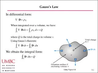
Gauss’s Law • In differential form: • When integrated over a volume, we have • where Q is the total charge in volume v. • Using Gauss’s theorem: • We obtain the integral form: Ulaby Figure 4-8
Gauss’s Law • Applications • In some simple cases with high symmetry, solutions may be found directly • A point charge • — This just reproduces Coulomb’s law • A line charge • A planar charge Ulaby Figure 4-9 — We obtained this result earlier by direct integration
Gauss’s Law • Applications • The line charge in more detail: — From symmetry, • Only the r-component of D is present, and it points in the r-direction • We consider a cylinder of height h surrounding the line charge. It contains a charge Q = rlh • We thus find • which implies • from which we conclude Ulaby Figure 4-10
Gauss’s Law • Applications • An even more important application of the integral formulation in today’s world is to serve as the starting point for numerical approaches!
The Scalar Potential — Voltage • Physical Meaning • The voltage V between two points indicates the work (energy) required to move a unit charge from the first point to the second • The field exerts a force Fe = qE on the charge. An external source of energy — like a battery — is required to move the charges; the external force must counteract the electrical force; Fext = –Fe = –qE. • We have Ulaby Figure 4-11
The Scalar Potential — Voltage • Physical Meaning • The voltage V between two points is independent of the path that is used to go between those two points • This is the source of: Kirchhoff’s Voltage Law • An important consequence: • In an axiomatic approach, we may derive this result from the second equation of electrostatics: ×E = 0. • Using Stokes theorem, we have Ulaby Figure 4-12
The Scalar Potential — Voltage • Physical Meaning • More generally, ×E 0 due to a changing magnetic field and Kirchoff’slaw breaks down! • The Concept of Ground • Voltage is defined as the potential difference between two points. • To set an absolute voltage reference, we assume that the voltage is zero in the ground, which corresponds to bringing a particle from . Ulaby Figure 4-12
The Scalar Potential — Voltage • Voltage due to Point Charges • From a single charge, using • From a charge q that is at R1 0, we have • For multiple charges Ulaby 2001
The Scalar Potential — Voltage • Voltage due to Continuous Distributions • By analogy with our earlier definition of the fields due to charge distributions, we have • Voltages are typically much easier to calculate than fields because there is just one scalar quantity to calculate instead of three vector components!
The Scalar Potential — Voltage • Calculating the Electric Field from the Voltage Field • From the equation dV = –E·dl , we infer • The preferred approach to calculating the field is to first determine the voltage field and then use the equation E = –V to determine the electric field
The Scalar Potential — Voltage Electric Dipole: Ulaby Example 4-7 (extended to arbitrary distances) Question: An electric dipole has two charges with same the same magnitude and the opposite sign separated by a distance d. Determine the voltage and the field Answer: In contrast to Ulaby’s example, wecalculate the field at any distance. We start withcylindrical coordinates, which are more convenientwhen the distances are arbitrary. We have Ulaby Figure 4-13
The Scalar Potential — Voltage Electric Dipole: Ulaby Example 4-7 (extended to arbitrary distances) Answer (continued): We note that the field is independent of f. So, the electric field becomes Ulaby Figure 4-13
The Scalar Potential — Voltage Electric Dipole: Ulaby Example 4-7 (extended to arbitrary distances) Answer (continued): In spherical coordinates, we have In the limit
The Scalar Potential — Voltage Electric Dipole: Ulaby Example 4-7 (extended to arbitrary distances) Answer (continued): We conclude Note the cubic falloff with distance and the proportionality to the charge separation! This behavior is characteristic of dipoles.
Electrical Properties of Materials • Conductors and Dielectrics • In electromagnetic theory, we treat materials as conductors or dielectrics • In conductors, the charges and currents appear in r and J. • In dielectrics, the charges and currents appear in e and m. • What about semiconductors? • The answer is complicated. It depends on • The material properties • Electric field properties; particularly the frequency • It can be useful to treat different currents and charges in the same material differently; there can be both bound and free charges and currents in the same medium.
Conductance and Resistance • Ohm’s Law: • The simplest model that relates the current to the electric field is Ohm’s law, • J = sE • Two important limits: • A perfect (ideal) conductor; s = , E = 0. • A perfect (ideal) dielectric; s = 0, J = 0. • Real materials can be more complicated; other effects can include • A tensor response or a nonlinear response. • A portion of the current that is due to the magnetic field.
Conductance and Resistance • Conductivity and Resistance: • We may relate the conductivity and the resistance in a wire of length l and area A: • From the relation V = IR, we conclude R = l /sA NOTE: Conductance is defined as G = 1/R Ulaby Figure 4-13
Conductance and Resistance Conductance of a coaxial cable: Ulaby Example 4-9 Question: We are now ready to derive the transmission line parameter G for the coaxial cable geometry. This is the first transmission line parameter that we will derive! A coaxial cable of length l has inner and outer conductors of radius a and b and an insulating layer with a conductivity s. What is G ? Answer: Let I be the current that flows from the inner conductor to the outer conductor. At any distance r, the area through which the current flows isA = 2prl. We now have, Ulaby Figure 4-15
Conductance and Resistance Conductance of a coaxial cable: Ulaby Example 4-9 Answer (continued): We now have, from which we conclude Ulaby Figure 4-15
Conductance and Resistance • Joule’s Law: Power dissipation in a resistor • From basic mechanical theory, we have • where • FV = the average force acting on a small volume of charges • uV = the average drift velocity of a small volume of charges • and we use • from which we may integrate to obtain • This relationship is general. When Ohm’s law holds • In the one-dimensional geometry for an electrical wire, This explains the standard circuit formulae for power dissipation!
Tech Brief 7: Resistive Sensors • Electrical Sensors • Respond to applied stimulus by generating an electrical signal • Electrical signal changes depending on intensity of stimulus • Voltage, current, or other attribute • Stimuli include physical, chemical, biological quantities • Temperature, pressure, position, distance, motion, velocity, aceleration, concentration (gas or liquid), blood flow, etc. • Types of sensors • Resistive • Capacitive, inductive, emf sensors (covered later)
Tech Brief 7: Resistive Sensors • Piezoresistivity • Stretching a conductor by an external force decreases A and increases l • Greek work piezein means to press • Resistance relationship approximately modeled by a linear equation, where a0 is the piezoresistive coefficient
Boundary Conditions Field Decomposition: We first decompose the fields in media 1 and 2, indicated E1 and E2 into tangential and normal components field decomposition intotangential and normal components tangential boundary conditions normal boundary conditions Ulaby Figure 4-18
Boundary Conditions • Tangential conditions: • We follow the path abcdashown in the figure, we use , and we let Dh 0. We also note that in this limit, |b–a| = |d–c| = Dl. We have • We conclude: field decomposition intotangential and normal components tangential boundary conditions normal boundary conditions Ulaby Figure 4-18
Boundary Conditions • Normal conditions: • We use Gauss’s law on the bottom and top of the pill box in the figure, • Along with the relation , to obtain field decomposition intotangential and normal components tangential boundary conditions normal boundary conditions Ulaby Figure 4-18
Boundary Conditions Application of Boundary Conditions: Ulaby Example 4-10 Question: The x-y plane at z = 0 is a charge-free boundary separating two dielectric media with permittivities e1 and e2. If the electric field in medium 1 is find the electric field E2 in medium 2 and the anglesq1 and q2. Answer: Let From the boundary conditions, we have We conclude Ulaby Figure 4-19
Boundary Conditions Application of Boundary Conditions: Ulaby Example 4-10 Answer (continued): The tangential and normal components of E1 and E2 are given by from which we infer The angles are related by Ulaby Figure 4-19
Boundary Conditions • Dielectric-Conductor Interface: • If medium 2 is the conductor, then we have E2 = 0 and D2 = 0 everywhere — including the interface with medium 1 • It follows that • which can be combined to yield • Field lines are always normal to thesurface of a conductor! Ulaby Figure 4-21
Capacitance • We are now ready to derive the capacitances that we used in the section on transmission lines • Basic theory: • When a voltage is applied between two conductors, the conductors accumulate an equal and opposite charge that distributes itself so that the surface is at a single potential and there is no electric field to move charges on the surface. • Definition of capacitance: C = Q/V • The electric field at the surface of a conductor is given by Ulaby Figure 4-23
Capacitance • Basic theory: • On the +V surface, we have • The voltage V is related to E by • where P1 is on the +V conductor and P2 is on the –V conductor • We conclude: Ulaby Figure 4-23
Capacitance • Relation of Resistance and Capacitance: • When the material between the conductors has conductivity s, we found earlier (slide 9.17) • When s and e are uniform, it follows: RC = e /s. • Hence, if we know one, we can find the other! • Example: A coaxial cable.We showed earlier (slide 9.19): R = ln(b/a) /2psl . It follows thatC = 2pel /ln(b/a) .
Tech Brief 8: Supercapacitors as Batteries • Electrochemical double-layer capacitor (EDLC) • Energy storage process a hybrid of capacitor and electrochemical voltaic battery • Batteries store more energy that capacitors, but capacitors charge and discharge more rapidly. • Energy density (measured in watt-hours per kg) lower for capacitors and supercapacitors compared to batteries • Power density is opposite case
Boundary Conditions Parallel Plate Capacitor: Ulaby Example 4-11 Question: Find the capacitance of a parallel plate capacitor in which each plate has surface area A and they are separated by a distance d. Ignore the fringing fields that appear in any real capacitor. Answer: On the upper plate, we have rS = Q / A. It follows that . We also have We conclude: Ulaby Figure 4-24
Electrostatic Energy • Work performed in charging a capacitor: • The charges already on a capacitor repel new charges that are added. Work must be done to add the new charges. The voltage on the capacitor is related to its charge by the relation: V = q / C. The increment of work that is required to add an increment of charge is: dWe = Vdq = (q /C) dq. We conclude that • Field Energy • The energy may be written in terms of the electric field as
Electrostatic Energy • Field Energy • We now define an electrostatic potential energy density as • The electrostatic potential energy generalizes to • in any geometry. We can use this energy to do work on other charges. • Where is the energy? • Is it in the fields or in the charges?
Tech Brief 9: Capacitive Sensors • Capacitive sensors respond to changes in geometry (space between conductors) or dielectric effects (changes in the insulator between conductors) • Field gauge • Sensitive to permittivity changes • Humidity Sensor • Patterned to enhance A/d ratio • Relative humidity affects air • permittivity
Tech Brief 9: Capacitive Sensors • Capacitive sensors respond to changes in geometry (space between conductors) or dielectric effects (changes in the insulator between conductors) • Pressure Sensor • Two capacitors in series • Noncontact Sensor • Senses objects near conductors
Tech Brief 9: Capacitive Sensors • Capacitive sensors respond to changes in geometry (space between conductors) or dielectric effects (changes in the insulator between conductors) • Fingerprint Imager • Two dimensional array of capacitive sensors • Records electrical representation of fingerprint
Assignment • Reading:Ulaby, Chapter 5 • Problem Set 4: Some notes. • There are 9 problems. As always, YOU MUST SHOW YOUR WORK TO GET FULL CREDIT! • Please watch significant digits. • Get started early!