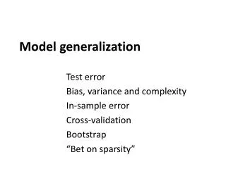

Model generalization
E N D
Presentation Transcript
Model generalization Brief summary of methods Bias, variance and complexity Brief introduction to Stacking
Brief summary Capability to learn highly abstract representations Need expert input to select representations Shallow classifiers (linear machines) Parametric Nonlinear models Kernel machines Deep neural networks “Do not generalize well far from the training examples” Linear partition Nonlinear partition Flexible Nonlinear partition Extract higher order information
Model Training data Testing data Model Testing error rate Training error rate Good performance on testing data, which is independent from the training data, is most important for a model. It serves as the basis in model selection.
Test error To evaluate prediction accuracy, loss functions are needed. Continuous Y: In classification, categorical G (class label): Where , Except in rare cases (e.g. 1 nearest neighbor), the trained classifier always gives a probabilistic outcome.
Test error The log-likelihood can be used as a loss-function for general response densities, such as the Poisson, gamma, exponential, log-normal and others. If Prθ(X)(Y) is the density of Y , indexed by a parameter θ(X) that depends on the predictor X, then The 2 makes the log-likelihood loss for the Gaussian distribution match squared error loss.
Test error Test error: The expected loss over an INDEPENDENT test set. The expectation is taken with regard to everything that’s random - both the training set and the test set. In practice it is more feasible to estimate the testing error given a training set: Training error is the average Loss over just the training set:
Test error Test error for categorical outcome: Training error:
Goals in model building Model selection: Estimating the performance of different models; choose the best one (2) Model assessment: Estimate the prediction error of the chosen model on new data.
Goals in model building Ideally, we’d like to have enough data to be divided into three sets: Training set: to fit the models Validation set: to estimate prediction error of models, for the purpose of model selection Test set: to assess the generalization error of the final model A typical split:
Goals in model building What’s the difference between the validation set and the test set? The validation set is used repeatedly on all models. The model selection can chase the randomness in this set. Our selection of the model is based on this set. In a sense, there is over-fitting in terms of this set, and the error rate is under-estimated. The test set should be protected and used only once to obtain an unbiased error rate.
Goals in model building In reality, there’s not enough data. How do people deal with the issue? Eliminate validation set. Draw validation set from training set. Try to achieve generalization error and model selection. (AIC, BIC, cross-validation ……) Sometimes, even omit the test set and final estimation of prediction error; publish the result and leave testing to later studies.
Bias-variance trade-off In the continuous outcome case, assume The expected prediction error in regression is:
Bias-variance trade-off Kernel smoother. Green curve-truth. Red curves – estimates based on random samples.
Bias-variance trade-off K-nearest neighbor classifier: The higher the k, the lower the model complexity (estimation becomes more global, space partitioned into larger patches) Increase k, the variance term decreases, and the bias term increases. (Here x’s are assumed to be fixed; randomness only in y) Bias
Bias-variance trade-off For linear model with p coefficients, The average of ||h(x0)||2 over sample values is p/N Model complexity is directly associated with p.
Bias-variance trade-off An example. 50 observations, 20 predictors, uniformly distributed in the hypercube [0, 1]20 Y is 0 if X1 ≤ 1/2 and 1 if X1 > 1/2, and apply k-nearest neighbors. Red: prediction error Green: squared bias Blue: variance
Bias-variance trade-off An example. 50 observations, 20 predictors, uniformly distributed in the hypercube [0, 1]20 Red: prediction error Green: squared bias Blue: variance
Stacking Increase the model space Ensemble learning Combining weak learners Combining strong learners Bagging Stacking Boosting Random forest
Stacking Strong learner ensembles (“Stacking” and beyond): CurrentBioinformatics, 5, (4):296-308, 2010.
Stacking • Uses cross validation to assess the individual performance of prediction algorithms • Combines algorithms to produce an asymptotically optimal combination For each predictor, predict each observation in a V-fold cross-validation Find a weight vector: Combine the prediction from individual algorithms using the weights. Stat in Med. 34:106–117
Stacking Lancet Respir Med. 3(1):42-52