Download
1 / 39
420 likes | 664 Vues
Chapter 14 Finite Impulse Response (FIR) Filters. Learning Objectives. Introduction to the theory behind FIR filters: Properties (including aliasing). Coefficient calculation. Structure selection. Implementation in Matlab, C, assembly and linear assembly. Introduction.

E N D
Chapter 14 Finite Impulse Response (FIR) Filters
Learning Objectives • Introduction to the theory behind FIR filters: • Properties (including aliasing). • Coefficient calculation. • Structure selection. • Implementation in Matlab, C, assembly and linear assembly.
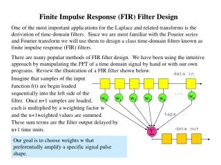
Introduction • Amongst all the obvious advantages that digital filters offer, the FIR filter can guarantee linear phase characteristics. • Neither analogue or IIR filters can achieve this. • There are many commercially available software packages for filter design. However, without basic theoretical knowledge of the FIR filter, it will be difficult to use them.
Properties of an FIR Filter • Filter coefficients: x[n] represents the filter input, bk represents the filter coefficients, y[n] represents the filter output, N is the number of filter coefficients (order of the filter).
Properties of an FIR Filter • Filter coefficients: FIR equation Filter structure
Properties of an FIR Filter • Filter coefficients: • If the signal x[n] is replaced by an impulse [n] then:
Properties of an FIR Filter • Filter coefficients: • If the signal x[n] is replaced by an impulse [n] then:
Properties of an FIR Filter • Filter coefficients: • If the signal x[n] is replaced by an impulse [n] then:
Properties of an FIR Filter • Filter coefficients: • Finally:
Properties of an FIR Filter • Filter coefficients: With: • The coefficients of a filter are the same as the impulse response samples of the filter.
Frequency Response of an FIR Filter • By taking the z-transform of h[n], H(z): • Replacing z by ej in order to find the frequency response leads to:
Frequency Response of an FIR Filter • Since e-j2k = 1 then: • Therefore: • FIR filters have a periodic frequency response and the period is 2.
Frequency Response of an FIR Filter x[n] FIR y[n] Fs/2 • Frequency response: x[n] y[n] Freq Freq Fs/2
Frequency Response of an FIR Filter Fs/2 • Solution: Use an anti-aliasing filter. x[n] x(t) ADC FIR y[n] Analogue Anti-Aliasing x(t) y[n] Freq Freq Fs/2
Phase Linearity of an FIR Filter • A causal FIR filter whose impulse response is symmetrical is guaranteed to have a linear phase response. Even symmetry Odd symmetry
Phase Linearity of an FIR Filter • A causal FIR filter whose impulse response is symmetrical (ie h[n] = h[N-1-n] for n = 0, 1, …, N-1) is guaranteed to have a linear phase response.
Phase Linearity of an FIR Filter 90o delay 90o delay • Application of 90° linear phase shift: IH I + Reverse + Signal separation - Forward Q + QH
Design Procedure • To fully design and implement a filter five steps are required: (1) Filter specification. (2) Coefficient calculation. (3) Structure selection. (4) Simulation (optional). (5) Implementation.
Coefficient Calculation - Step 2 • There are several different methods available, the most popular are: • Window method. • Frequency sampling. • Parks-McClellan. • We will just consider the window method.
Window Method • First stage of this method is to calculate the coefficients of the ideal filter. • This is calculated as follows:
Window Method • Second stage of this method is to select a window function based on the passband or attenuation specifications, then determine the filter length based on the required width of the transition band. Using the Hamming Window:
Window Method • The third stage is to calculate the set of truncated or windowed impulse response coefficients, h[n]: for Where: for
Window Method close all; clear all; fc = 8000/44100; % cut-off frequency N = 133; % number of taps n = -((N-1)/2):((N-1)/2); n = n+(n==0)*eps; % avoiding division by zero [h] = sin(n*2*pi*fc)./(n*pi); % generate sequence of ideal coefficients [w] = 0.54 + 0.46*cos(2*pi*n/N); % generate window function d = h.*w; % window the ideal coefficients [g,f] = freqz(d,1,512,44100); % transform into frequency domain for plotting figure(1) plot(f,20*log10(abs(g))); % plot transfer function axis([0 2*10^4 -70 10]); figure(2); stem(d); % plot coefficient values xlabel('Coefficient number'); ylabel ('Value'); title('Truncated Impulse Response'); figure(3) freqz(d,1,512,44100); % use freqz to plot magnitude and phase response axis([0 2*10^4 -70 10]); • Matlab code for calculating coefficients:
Window Method 0.4 0.3 0.2 0.1 0 -0.1 0 20 40 60 80 100 120 140 Truncated Impulse Response h(n) Coefficient number, n
Realisation Structure Selection - Step 3 • Direct form structure for an FIR filter:
Realisation Structure Selection - Step 3 • Direct form structure for an FIR filter: • Linear phase structures: • N even: • N Odd:
Realisation Structure Selection - Step 3 (a) N even. (b) N odd.
Realisation Structure Selection - Step 3 • Direct form structure for an FIR filter: • Cascade structures:
Realisation Structure Selection - Step 3 • Direct form structure for an FIR filter: • Cascade structures:
Implementation - Step 5 • Implementation procedure in ‘C’ with fixed-point: • Set up the codec (\Links\CodecSetup.pdf). • Transform: to ‘C’ code. (\Links\FIRFixed.pdf) • Configure timer 1 to generate an interrupt at 8000Hz (\Links\TimerSetup.pdf). • Set the interrupt generator to generate an interrupt to invoke the Interrupt Service Routine (ISR) (\Links\InterruptSetup.pdf).
Implementation - Step 5 • Implementation procedure in ‘C’ with floating-point: Same set up as fixed-point plus: • Convert the input signal to floating-point format. • Convert the coefficients to floating-point format. • With floating-point multiplications there is no need for the shift required when using Q15 format. • See \Links\FIRFloat.pdf
Implementation - Step 5 • Implementation procedure in assembly: Same set up as fixed-point, however: • is written in assembly. (\Links\FIRFixedAsm.pdf) • The ISR is now declared as external.
Implementation - Step 5 • #pragma DATA_ALIGN (symbol, constant (bytes)) • Implementation procedure in assembly: The filter implementation in assembly is now using circular addressing and therefore: • The circular pointers and block size register are selected and initialised by setting the appropriate values of the AMR bit fields. • The data is now aligned using: • Set the initial value of the circular pointers, see \Links\FIRFixedAsm.pdf.
Implementation - Step 5 b0 x0 b1 x1 b2 x2 b3 x3 y[n] time 0 1 2 y0 = b0*x0 + b1*x1 + b2*x2 + b3*x3 Circular addressing link slide.
Implementation - Step 5 b0 b1 b2 b3 y[n] time 0 1 2 x4 x1 x2 x3 y0 = b0*x0 + b1*x1 + b2*x2 + b3*x3 y1 = b0*x4 + b1*x1 + b2*x2 + b3*x3 Circular addressing link slide.
Implementation - Step 5 b0 b1 b2 b3 y[n] time 0 1 2 x4 x5 x2 x3 y0 = b0*x0 + b1*x1 + b2*x2 + b3*x3 y1 = b0*x4 + b1*x1 + b2*x2 + b3*x3 y2 = b0*x4 + b1*x5 + b2*x2 + b3*x3 Circular addressing link slide.
FIR Code • Code location: • Code\Chapter 14 - Finite Impulse Response Filters • Projects: • Fixed Point in C: \FIR_C_Fixed\ • Floating Point in C: \FIR_C_Float\ • Fixed Point in Assembly: \FIR_Asm_Fixed\ • Floating Point in Assembly: \FIR_Asm_Float\
Chapter 14 Finite Impulse Response (FIR) Filters - End -