
SlideServe
Menu
Préférences
© SlideServe · v2026

Overview of Supervised Learning

sydnee avatar
14 diapositives · 328 Views · Sep 03, 2014

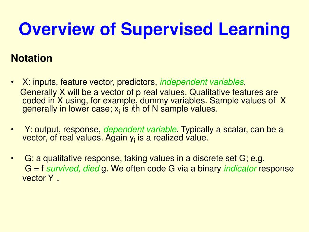
Notation X: inputs, feature vector, predictors, independent variables . Generally X will be a vector of p real values. Qualitative features are coded in X using, for example, dummy variables. Sample values of X generally in lower case; x i is i th of N sample values.
Overview of Supervised Learning - slide 1
01 / 14Overview of Supervised Learning
1 / 17

Télécharger la présentation

Overview of Supervised Learning
Une image / un lien ci-dessous est fourni (tel quel) pour télécharger la présentation

Politique de téléchargement : le contenu du site vous est fourni TEL QUEL pour votre information et votre usage personnel ; il ne peut être vendu, concédé sous licence ni partagé sur d’autres sites sans l’accord de son auteur.Le contenu vous est fourni TEL QUEL, pour votre information et votre usage personnel uniquement. Téléchargez la présentation en cliquant sur ce lien. Lors du téléchargement, si vous ne parvenez pas à télécharger une présentation, l’éditeur a peut-être supprimé le fichier de son serveur.Pendant le téléchargement, si vous ne parvenez pas à obtenir une présentation, le fichier a peut-être été supprimé par l’éditeur.

F I N

Plus de contenu associé

Transcription de la présentation
  1. Notation X: inputs, feature vector, predictors, independent variables. Generally X will be a vector of p real values. Qualitative features are coded in X using, for example, dummy variables. Sample values of X generally in lower case; xi is ith of N sample values. Y: output, response, dependent variable. Typically a scalar, can be a vector, of real values. Again yi is a realized value. G: a qualitative response, taking values in a discrete set G; e.g. G = fsurvived, diedg. We often code G via a binary indicator response vector Y . Overview of Supervised Learning

  2. 200 points generated in R2 from an unknown distribution; 100 in each of two classes G = fGREEN; REDg. Can we build a rule to predict the color of future points?

  3. Linear Regression

  4. Possible Scenarios • Scenario 1: The data in each class are generated from a Gaussian distribution with uncorrelated components, same variances, and different means. • Scenario 2: The data in each class are generated from a mixture of 10 gaussians in each class. • For Scenario 1, the linear regression rule is almost optimal (Chapter 4). • For Scenario 2, it is far too rigid.

  5. K-Nearest Neighbors

  6. 15-nearest neighbor classification. Fewer training data are misclassified, and the decision boundary adapts to the local densities of the classes.

  7. 1-nearest neighbor classification. None of the training data are misclassified.

  8. Discussion • Linear regression uses 3 parameters to describe its fit. K-nearest neighbors uses 1, the value of k? • More realistically, k-nearest neighbors uses N/k effective number of parameters Many modern procedures are variants of linear regression and K-nearest neighbors: • Kernel smoothers • Local linear regression • Linear basis expansions • Projection pursuit and neural networks

  9. Linear regression vs k-nn? • First we expose the oracle. The density for each class was an equal mixture of 10 Gaussians. • For the GREEN class, its 10 means were generated from a • N((1; 0)T ; I) distribution (and considered fixed). • For the RED class, the 10 means were generated from a • N((0; 1)T ; I) distribution. The within cluster variances were 1/5. • See page 17 for more details, or the book website for the actual data.

  10. The results of classifying 10,000 test observations generated from this distribution. The Bayes Erroris the best performance possible.

  11. Statistical Decision TheoryCase 1: Quantitative Output Y

  12. Statistical Decision TheoryCase 2: Qualitative Output G

  13. This is known as the Bayes classifier. It just says that we should pick the class having maximum probability at the input X Question: how do we construct the Bayes classifier for our simulation example?