Download

1 / 31
450 likes | 1.15k Vues
Introduction to Finite Element Analysis for Structure Design. Dr. A. Sherif El-Gizawy. Elasticity Principles. F : Applied Force & A : Area l : Initial Length Stress = = F/ A dl= displacement (deformation) Strain = = dl/l. l. A. d l. F. Stress-Strain Relation (Hooke’s Law)

E N D
Introduction to Finite Element Analysis for Structure Design Dr. A. Sherif El-Gizawy
Elasticity Principles • F: Applied Force & A : Area • l : Initial Length • Stress = = F/ A • dl= displacement (deformation) • Strain = = dl/l l A dl F
Stress-Strain Relation(Hooke’s Law) • Modulus of Elasticity = • E = / • = E * x in the x-direction • = /E Elastic Deformation Zone • Plastic Work (Deformation Energy) • Plastic Work/ Unit Volume =dW = F x dl/Volume • =F x dl/ (A x l) = x • dW = x
3D Stress-Strain Relationship x= 1/E*((x- (y + z)) Where x :normal strain along x direction : Poisson Ration Shear Strain, xy = xy/ G xy: Shear Stress G : Shear Modulus of Elasticity
Effective Stress (Von-Mises) = ((x- y)2 + (y- z)2 + (z- x)2)1/2 when reaches a certain value (yield stress), the applied stress state will cause yielding Effective Strain = ( (x2+ y2+ z2))1/2
FEM Solution for Structural Design = E X (Hooke’s Law) F = A X(E X) = A XE (l /l) l l K A F = (A XE/l) Xl This is an analogy to spring Force with l l F A x E/l = Element Stiffness = Keq F Fsp = K x l F = KeqXl F = KeqXl
Element Stiffness = A x E/l = K eq • The Applied force F is given. • Deformation (deflection or displacement) l = F / Keq = Strain = l /l (calculated) = Stress = E x
Introduction to the Finite Element Method • Typically, for the structural stress analysis, it is required to determine the stresses and deformation (strains) throughout the structure which is in equilibrium and is subjected to applied loads. • The finite element method involves modeling of the structure using small units (finite elements). • A displacement function is associated with each finite element. The followings are the steps used in finite element method. This will be followed by illustration of the application of these steps on springs and plane stress cases.
Developing a Model for Finite Element Analysis The problem to be solved is specified in a) the physical domain and b) the discretized domain used by FEA
Line Element Two-dimensional Elements Three-dimensional Elements Axisymmmetric Element
Step 1. Discretize and Select Element Types Divide the structure into an equivalent system of finite elements with associated nodes. The simplest line elements, Fig.1.a has two nodes, one at each end. The basic two-dimensional elements, Fig. 1.b are loaded by forces in their own plane (plane stress). They are triangular or quadrilateral elements. The common three dimensional elements, Fig.1.c, are tetrahedral and hexahedral (brick) elements. They are used to perform three dimensional stress analysis in 3-D solid bodies.
Step 2. Select a Displacement Function • Choose a displacement function within each element using the nodal values of the element. Linear, quadratic, and polynomials are frequently used functions. • Step 3. Define the Stress/Strain Relationships • = dl/l • = E
Step 4. Derive the Element Stiffness Matrix and Equations • The stiffness matrix and element equations relating nodal forces and displacements are obtained using force equilibrium conditions or the principle of minimum potential energy. • Step 5. Assemble the Element Equations to obtain the Global Equations • Step 6. Solve for the Unknown Displacements • Step 7. Solve for the Element Strains and Stresses • Step 8. Interpret the Results • The final goal is to interpret and analyze the results for use in the design process.
Von Mises stress in ¼ model of thin plate under tension using 1st order elements A disaster waiting to happen using first order elements
A mesh of tetrahedral p-elements produced by MECHANICA A mesh of solid tetrahedral (4 nodes) h-elements
Steps in FEA using Pro-Mechanica • Step 1: Draw part in Pro-Engineer • Step 2: Start Pro-Mechanica • Step 3: Choose the Model Type • Step 4: Apply the constraints • Step 5: Apply the loads • Step 6: Assign the material • Step 7: Run the Analysis • Step 8: View the results by post-processing
Step 1: Creation of the part • Use Protrusion by Sweep to create this part (bar.prt)
Step 2: Starting Pro-Mechanica • In Pro-Engineer window, go to Applications Mechanica to start Pro-Mechanica. • The part (bar.prt) will be loaded in Pro-Mechanica with a new set of icons for Structural, thermal Analysis
Step 3: Choosing the model type • In Mechanica menu, select • Structure Model Model Type • Four different models can be created: • 3D Model • Plane Stress • Plane Strain • 2D Axisymmetric • We will select 3D Model
Step 4: Applying the Constraints • Create a new constraint by • Model Constraints New Surface • Give a name for the constraints (fixed_face) and select the surface to be constrained • Specify the constraints (in our case will be fixed for all degrees of freedom) • Preview and press Ok
Step 5: Applying the loads • Similar to Constraints, create a new load by Model Load New Surface • Give a name for the applied load (endload) • Select the surface where the load will be applied • Specify the loads (Fx:500, Fy:-250, Fz:0) • Preview and press Ok
Step 6: Assigning the material • Model Materials • A window will pop up with the list of Pro-Mechanica materials. Add the required material and then assign the material to the part. • Click on Edit if any change in material properties are to be made. • Press Ok
Step 7: Running the Analysis • In Mechanica menu, select Analysis • Select File New Static in “Analysis and Design Studies” dialog box and give a name for the analysis (bar). • The constraints and loads are automatically loaded. • In Convergence tab, select Quick Check to check for errors and then select Multi-pass adaptive for the reliable and accurate results. Change the order of the polynomial and percentage of convergence as required. • Finally, click on Run icon to start the analysis (click on Display Study Status to view the current status and completion of the analysis)
Step 8: Viewing the results • For post-processing, select Results from Pro-Mechanica window • A new window will open, and click on “Insert a New Definition” icon. In the dialog box, select the folder where the analysis is saved. • Select Fringe as Display type, Stress as Quantity and von-mises as the stress component to display • Similarly, other quantities can be displayed in one window.