Download

1 / 22
260 likes | 698 Vues
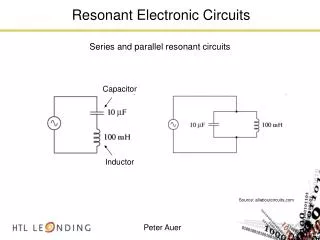
ANALOG ELECTRONIC CIRCUITS 1. EKT 204 Frequency Response of BJT Amplifiers (Part 2). Small capacitances exist between the base and collector and between the base and emitter. These effect the frequency characteristics of the circuit. HIGH FREQUENCY.

E N D
ANALOG ELECTRONIC CIRCUITS 1 EKT 204 Frequency Response of BJT Amplifiers (Part 2)
Small capacitances exist between the base and collector and between the base and emitter. These effect the frequency characteristics of the circuit. HIGH FREQUENCY • The gain falls off at high frequency end due to the internal capacitances of the transistor. • Transistors exhibit charge-storage phenomena that limit the speed and frequency of their operation. reverse-biased junction capacitance C = Cbe------2 pF ~ 50 pF forward-biased junction capacitance C= Cbc------0.1 pF ~ 5 pF
Basic data sheet for the 2N2222 bipolar transistor Output capacitance Cob = Cbc Cib = Cbe Input capacitance
Miller’s Theorem • This theorem simplifies the analysis of feedback amplifiers. • The theorem states that if an impedance is connected between the input side and the output side of a voltage amplifier, this impedance can be replaced by two equivalent impedances, i.e. one connected across the input and the other connected across the output terminals.
I1 I2 V1 V2 Miller Equivalent Circuit Impedance Z is connected between the input side and the output side of a voltage amplifier..
V1 V2 Miller Equivalent Circuit (cont) .. The impedance Z is being replaced by two equivalent impedances, i.e. one connected across the input (ZM1) and the other connected across the output terminals (ZM2)
C I1 I2 V1 V2 Miller Capacitance Effect CM = Miller capacitance Miller effect Multiplication effect of Cµ
C + r V C gmV ro - C = Cbe C= Cbc High-frequency hybrid- model
r C CMi ro CMo gmV High-frequency hybrid- model with Miller effect A : midband gain
VCC = 10V R1 RC C2 22 k 2.2 k RS C1 10 F RL 600 10 F 2.2 k vS R2 RE C3 4.7 k 10 F 470 High-frequency in Common-emitter Amplifier Calculation Example Given : = 125, Cbe = 20 pF, Cbc = 2.4 pF, VA = 70V, VBE(on) = 0.7V vO • Determine : • Upper cutoff frequencies • Dominant upper cutoff frequency
RS vo vs R1||R2 C CMi r ro RC||RL CMo gmV High-frequency hybrid- model with Miller effect for CE amplifier midband gain Miller’s equivalent capacitor at the input Miller’s equivalent capacitor at the output
Calculation (Cont..) Thevenin’s equivalent resistance at the input Thevenin’s equivalent resistance at the output total input capacitance total output capacitance upper cutoff frequency introduced by input capacitance upper cutoff frequency introduced by output capacitance
How to determine the dominant frequency • The lowestof the two values of upper cutoff frequencies is the dominant frequency. • Therefore, the upper cutoff frequency of this amplifier is
A (dB) ideal Amid -3dB actual f (Hz) fC4 fC5 fC1 fC2 fC3 fL fH TOTAL AMPLIFIER FREQUENCY RESPONSE
VCC = 5V R1 RC C2 33 k 4 k RS C1 2 F RL 2 k 1 F 5 k vS R2 RE C3 22 k 10 F 4 k Total Frequency Response of Common-emitter Amplifier Calculation Example Given : = 120, Cbe = 2.2 pF, Cbc = 1 pF, VA = 100V, VBE(on) = 0.7V vO • Determine : • Midband gain • Lower and upper cutoff frequencies
Step 4 - Lower cutoff frequency (fL) Due to C1 Due to C2 Due to C3 SCTC method Lower cutoff frequency
Step 5 - Upper cutoff frequency (fH) Miller capacitance Input & output resistances
Step 5 - Upper cutoff frequency (fH) Input side Output side Upper cutoff frequency (the smallest value)
Exercise • Textbook: Donald A. Neamen, ‘MICROELECTRONICS Circuit Analysis & Design’,3rd Edition’, McGraw Hill International Edition, 2007 • Exercise 7.11