Download
1 / 100
1.09k likes | 1.77k Vues
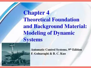
Chapter 4 Theoretical Foundation and Background Material: Modeling of Dynamic Systems. Automatic Control Systems, 9 th Edition F. Golnaraghi & B. C. Kuo. 0, p. 147. Main Objectives of This Chapter. To introduce modeling of mechanical systems To introduce modeling of electrical systems

E N D
Chapter 4Theoretical Foundation and Background Material: Modeling of Dynamic Systems Automatic Control Systems, 9th Edition F. Golnaraghi & B. C. Kuo
0, p. 147 Main Objectives of This Chapter • To introduce modeling of mechanical systems • To introduce modeling of electrical systems • To introduce modeling thermal & fluid systems • To discuss sensors and actuators • To discuss linearization of nonlinear systems • To discuss analogies
1, p. 148 4-1 Introduction to Modeling of Mechanical Systems • Mass: • Translation motion: a motion that takes places along a straight or curved path acceleration a, velocity v, displacement y • Newton’s law of motion: • Force equation:
1, p. 149 Linear Translation Motion • Mass: • Linear spring: • Friction for translation motion: • viscous friction, static friction, Coulomb friction preload tension
1, p. 150 Friction for Translation Motion (a) Viscous friction (b) Static friction (c) Coulomb friction
1, p. 151 Basic Translational Mechanical System
1, p. 152 Example 4-1-1 • Force equation: Transfer function:
1, p. 152 Example 4-1-1 (cont.) • Force equation: • State space form: with initial conditions without initial conditions
1, p. 154 Example 4-1-2 • Force equation: • Transfer function:
1, p. 155 Example 4-1-2 (cont.) • State equations:
1, p. 156 Example 4-1-3 State equations: State variables:
1, p. 157 Rotational Motion • Rotational motions: a motion about a fixed axis angular displacement , angular velocity , angular acceleration • Newton’s law of motion for rotational motion: • Inertia (J): a circular disk or shaft of radius r and mass M • Torque equation: a torque T is applied to a body with inertia J
1, p. 158 Torsional Spring & Friction • Torsional Spring: • Friction for Rotational Motion: • Viscous friction: • Static friction: • Coulomb friction: preload torque
1, p. 159 Basic Rotational Mechanical System
1, p. 158 Example 4-1-4 Torque or moment equation:
1, p. 160 Example 4-1-5 Torque equation:
1, p. 160 Example 4-1-5 (cont.) • Three energy-storage elements: Jm, JL, K 3 state variables • State variables: State equations:
1, p. 161 Conversion between Transiational and Rotational Motions • The equivalent inertia that the motor see: L: the lead of the screw equivalent
1, p. 162 Gear Train
1, p. 163 Gear Train with Friction and Inertia reflecting from gear 2 to gear 1 Figure 4-23
1, p. 164 Backlash and Dead Zone
2, p. 165 4-2 Introduction to Modeling Simple Electrical Systems
2, p. 166 Example 4-2-1 KVL: Current inC: State equations: State variables:
2, p. 166 Example 4-2-1 (cont.) State equations:
2, p. 167 Example 4-2-1 (cont.) • Transfer functions:
2, p. 168 Example 4-2-2 State variables
2, p. 169 Example 4-2-2 (cont.) Transfer functions:
2, p. 170 Example 4-2-3 Find the differential equation of the system.
2, p. 171 Example 4-2-4 Find the differential equation of the system
2, p. 172 Example 4-2-5 Node equation at e1:
3, p. 173 4-3 Modeling of Active Electrical Elements: Operational Amplifiers Idea Op-Amp: • The voltage between the + and terminals is zero. e+ = e, virtual ground or virtual short. • The currents into the + and terminals are zero. input impedance is infinite • The impedance seen looking into the output terminate is zero. the output is an idea voltage source. • eo = A(e+ e),gain A A
3, p. 174 Sum and Difference Negative sum Positive sum Difference
3, p. 174 First-Order Op-Amp Configirations 0 V
3, p. 175 Inverting Op-Amp Transfer Functions
3, p. 176 Table 4-4 (cont.)
3, p. 176 Example 4-3-1 Op-amp realization of PID controller: Proportional: Integral: Derivative: Output: Transfer function:
4, p. 177 4-4 Introduction to Modeling of Thermal Systems Elementary Heat Transfer Properties • Heat transfer is related to the heat flow rateq: • Capacitance (C): storage or (discharge) of heat in a body • The capacitance is related to the change of the body temperatureT with respective to time and the rate of heat flowq: • Three types of heat transfer: conduction, convection, or radiation. volume material density material specific heat
4, p. 178 Conduction • This type of heat transfer happens in solid materials due to a temperature difference between two surfaces. • Heat tends to travel from the hot to the cold region • One-direction heat conduction flow: k: Thermal conductivity related to the material used R: Thermal resistance A: Area normal to thedirection of heat flow x
4, p. 178 Convention • Convention occurs between a solid surface and a fluid exposed to it. h: the coefficient of convention heat transfer T = Tb Tf
4, p. 179 Radiation • The rate of heat transfer through radiation between two separate objects is determined by the Stephan-Boltzmann law, : Stephan-Boltzmann constant
4, p. 179 Table 4-5 Basic Thermal System Properties
4, p. 180 Example 4-4-1 Find the equations of heat transfer process = convention rate:
5, p. 181 4-5 Introduction to Modeling of Fluid Systems Elementary Fluid and Gas Properties • Mass flow rate: : fluid densityq: net fluid flow ratem: net mass flowqi: ingoing fluidqo: outgoing fluid
5, p. 181 Conservation of mass & Fluid Capacitance • Conservation of mass: • Capacitance – Incompressible Fluid:the ratio of the fluid flow rate q to the rate of pressure Mcv: mass of control volumeV: container volume 1. conservation of volume: 2. incompressible fluid:( is constant)
5, p. 182 Examples 4-5-1 & 4-5-2 • Example 4-5-1 The pressure in the tank: • Example 4-5-2 The pressure rate:
5, p. 183 Capacitance – Pneumatic Systems • Capacitance expresses the rate of change of the fluid mass with respect to pressure: • For a constant container: • Polytropic process: (n = 0 ~ : polytropic exponent) • Perfect gas law: (Rg: gas constant)
5, p. 183 General Gas Law • (the mass m is constant in a polytropic process) • For a constant temperature (an isothermal process): • For a constant pressure (an isobaric process): • For a constant volume (an isovolumetric process): • For a reversible adiabatic (an isentropic process): cp: the specific heat of gas at constant pressure cv: the specific heat of gas at constant volume
5, p. 184 Inductance – Incompressible Fluids • Inductance: fluid inertance in relation to the inertia of a moving fluid inside a passage (line or a pipe). • Newton’s second law: Fluid inductance
5, p. 184 Resistance – Incompressible Fluids • As in electrical systems, fluid resistors dissipate energy. • The force resisting the fluid passing through a passage: • Laminar flow: • Turbulent:
5, p. 185 Table 4-6: Resistance for Laminar Flows