Download
1 / 5
50 likes | 188 Vues
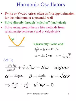
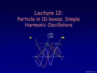
An Analytical Investigation of Piecewise-linear Harmonic Oscillators. Brendan Jones Christian Fadul. Introduction.

E N D
An Analytical Investigation of Piecewise-linear Harmonic Oscillators Brendan Jones Christian Fadul
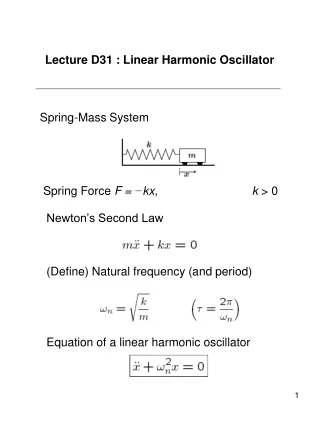
Introduction The equation of motion for a linear oscillator does not have a single analytical solution. As the components of the system in motion make intermittent contact with each other, an interesting piecewise linear form is examined in the motion of the system. The system under consideration shows a single degree of freedom that is periodically forced. Due to the complexity of expressing the position as a function of time, the piecewise function was solved by using a numerical integrator.
Hand Calculations First we drew the FBD’s LMB: mx'' = -c(x') – h(x) + F cos(ωt) Mass normalized motion equation: x'' + ξ(x') + H(x) = A cos(ωt) Simplification for integrator: x1 = x x2 = x' x'1 = x2 x'2 = -ξ(x2) - H(x1) + A cos(ωt)
Experimental Results x’’ = (1/2)*(-(1/2)*ξ+(1/2)*sqrt(ξ^2-4*H))^2*exp((-(1/2)*ξ+(1/2)*sqrt(ξ^2-4*H))*x)*(-r*ξ^2*ω^2-sqrt(ξ^2-4*H)*ξ*r*ω^2+2*r*H*ω^2-2*r*H^2+2*A*H)*(-sqrt(ξ^2-4*H)*ξ+ξ^2-4*H)/((2*ξ^2*ω^2-8*H*ω^2+ξ^4-6*H*ξ^2+8*H^2-ξ^3*sqrt(ξ^2-4*H)+4*sqrt(ξ^2-4*H)*ξ*H)*H)+(1/2)*(-(1/2)*ξ-(1/2)*sqrt(ξ^2-4*H))^2*exp((-(1/2)*ξ-(1/2)*sqrt(ξ^2-4*H))*x)*(-r*ξ^2*ω^2+sqrt(ξ^2-4*H)*ξ*r*ω^2+2*A*H+2*r*H*ω^2-2*r*H^2)*(sqrt(ξ^2-4*H)*ξ+ξ^2-4*H)/((sqrt(ξ^2-4*H)*ξ+ξ^2-2*H+2*ω^2)*H*(ξ^2-4*H))+(-(H-ω^2)*cos(ω*x)*ω^2-sin(ω*x)*ω^3*ξ)*A/(ω^4+(ξ^2-2*H)*ω^2+H^2). As you can see, the analytical form of the acceleration expression is very complex.
Conclusion With the knowledge obtained throughout the course it is possible to derive the equations of motion for this system. Using specific conditions for the system, different situations can be observed and examined. Through the examination of each of the special conditions of the system, the entire process is automatically checked for its accuracy. In this specific case, the original derivation of the equation of motion agrees with the solution set that was obtained in the experimental calculations. Also, we can cross check with the work done by Kisliakov and Popov [1] and Arnold [2] to verify that the solution obtained matches the solution set of the previous research.