Navigating Without Locations: A Sensor Network Approach for Dynamic Human Navigation
This study presents a novel human navigation system utilizing sensor networks without relying on physical location information. Traditional models face challenges, including the inherent limitations of human speed and the frequent updates required in dynamic dangerous situations. Our system comprises four design principles centered around building a responsive road map, guiding navigation, and enhancing routing efficiency. We detail implementation experiences using 36 TelosB Motes and provide performance evaluations showing the effectiveness of our system in ensuring safety while optimizing path selection.

Navigating Without Locations: A Sensor Network Approach for Dynamic Human Navigation
E N D
Presentation Transcript
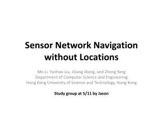
Sensor Network Navigation without Locations Mo Li, Yunhao Liu, Jiliang Wang, and Zheng Yang Department of Computer Science and Engineering Hong Kong University of Science and Technology, Hong Kong Study group at 5/11 by Jason
Outline • System introduction • Design principles • Implementation experience • Performance evaluation
System introduction • Traditional sensor network – data centric ,efficiently collecting, routing, and processing in-network sensory data. • Difference of human navigation network • no physically multicast or copied • Limited human speed • Frequent updating of emergency or dangerous situation changing
System introduction • Human navigation system based on sensor network with two characteristics: • Release the necessity of utilizing location information • Address the dynamic leading to variations of dangerous area
System introduction • Small-scale with 36 TelosB Motes on 802.15.4 • Objectives and requirements: • Safe: Be apart from dangerous area • Efficient: A shorter path is needed for rapid departure. • Scalable: Building and updating should be local and lightweight
Design principles • 4 components of designing principles: • Building the road map • Guiding navigation on the road map • Reacting to emergency dynamics • Improving routing efficiency
Building the road map • In 2D, the medial axis of a plane curve S is the locus of the centers of circles that are tangent to curve S in two or more points, where all such circles are contained in S. (It follows that the medial axis itself is contained in S.) Medial axis
Building the road map Medial axis are expressive and can capture the topological features of safe region R Un-sensed place are defined as dangerous area Preliminary information on boundary, like indoor environment, safely surrounded by walls or fences
Guiding navigation on the road map (1)Connecting the exit to the road map backbone - Defining potential field: p=1/d, extending each step on the most descending direction (2)Assigning directions on the road map - Flooding dc anddrfrom the gateway to all network (3)Exploring the routes for users - 3 stages, from cell to backbone, backbone routing and from gateway to exit (4)The safety of the navigation route -Guarantee maximizing the minimum distance from dangerous areas along the selected path
Reacting to emergency dynamics Expanding or shrinking of dangerous areas means points that switches in to or out from areas. Lemma 3.5. When the dangerous area in a cell c expands or shrinks continuously, only the points within c are affected Lemma 3.6. The emerging of a new dangerous point affects the points within the newly constructed cell and the diminishing of a dangerous point affects the points within the original cell. Theorem 3.7. The impact of the emergency dynamics in the field is local
Implementation experience s.danger is 0 when the node is out of dangerous area. s.borderis a booleanvariable that indicates whether the current node is on the boundary of the dangerous area s.mDist records the distance from the current node to the nearest dangerous area s.mSet records the set of nodes on the boundaries of dangerous areas that are of s.mDist to the current node s.roadis a booleanvariable that indicates whether the current node is on the road map backbone s.nextHop stores the ID of the next hop node along the path direction on the road. s.rDist records the minimum distance to the dangerous areas on the path from the current node to the exit
Implementation experience • Emergency happening deciding s.dangerand generate danger ID. • Confirming all boundary nodes(set s.border), and then flood to all network to decide s.mDistand s.mSet. • Examine s.mSet of all nodes to decide if it contains boundary modes on two or more dangerous areas(setting s.road)
Implementation experience • Calcculatings.potential=1/s.mDist • Gate way node flooding the exit information through the road backbone: • dc, which records the minimum number of hops to the dangerous areas along the road from the current node to the gateway, • dr, which records the number of hops along theroadfrom the current node to the gateway.
Implementation experience • Originally , every node sets its s.nextHopto be null, and s.rDist to be 0. • IF(s.rDist< dc), switches its s.nextHopto be the ID of the node that forwards the message and sets its s.rDist to be dc. • Assign dc as min(dc, s.mDist) and forward this message
Performance evaluation • Simulating randomly deploying sensor nodes with average node degree of 28 • Network size ranges from 1000 to 16000 • 10 internal users • Number of randomly inserting dangerous areas is uniformly chosen from 3 to 6.
Performance evaluation • SG=Skeleton Graph , PF=Potential Graph , RM=Road Map • A. Minimum Distance to the Danger: performance ratio=d/dOPT • B. Shortest Path: performance ratio= l/lOPT • C. Minimum Exposure Path: S=sum(1/dist^2), performance ratio =S/SOPT • D. Update Overhead