Download
1 / 43
430 likes | 551 Vues
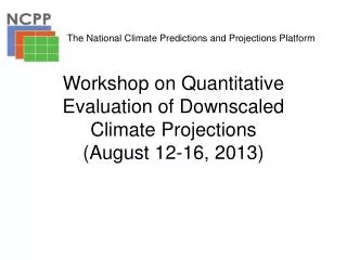
2013 Workshop on Quantitative Evaluation of Downscaled Data . “ Perfect Model” Experiments: Testing Stationarity in Statistical Downscaling (NCPP Protocol 2 ) is past performance an indication of future results ?.

E N D
2013 Workshop on QuantitativeEvaluation of Downscaled Data “Perfect Model” Experiments: Testing Stationarity in Statistical Downscaling (NCPP Protocol 2)is past performance an indication of future results? • Keith Dixon1, Katharine Hayhoe2, John Lanzante1, Anne Stoner2, AparnaRadhakrishnan3,V. Balaji4, Carlos Gaitán5 2 3 DRC Inc. 4 Princeton Univ. 5 Univ. of Oklahoma
Goals of this presentation • Define the ‘stationarity assumption’ inherent to statistical downscaling of future climate projections. • Present our ‘perfect model’ (aka ‘big brother’) approach to quantitatively assess the extent to which the stationarity assumption holds. • Illustrate with a few examples the kind of results one can generate using this evaluation framework (Anne Stoner will show more detail next…) • Introduce options to extend and supplement the method (setting the hurdleat different heights). • Invite statistical downscalers to consider testing their methods within the perfect model framework. • Garner feedback from workshop participants.
This project does not produce any data files that one would use in real world applications. The aim at GFDL is to gain knowledge about aspects of commonly used SD methods (& GCMS), and to communicate that knowledge so that better informed decisions can be made.
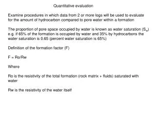
REAL WORLD APPLICATION: Cannot evaluate future skill -- left assuming transform functionsapply equally well to past & future -- “The Stationarity Assumption” Start with 3 types of data sets … lacking observations of the future Compute transform functions in training step (1 example below) Produce downscaled refinements of GCM (historical and/or future) Skill: Compare Obs to SD historical output (e.g., cross validation) TARGET ? ? ? PREDICTORS
“PERFECT MODEL” EXPERIMENTAL DESIGN: Start with 4 types of data sets – Hi-res GCM output as proxy for obs& coarsened version of Hi-res GCM output as proxy for usual GCM ? ? ? Proxy for observations in real-world applicationProxy for GCM output in real-world application
Daily time resolution~25km grid spacing194 x 114 grid22k pts
64:1 ~200km grid spacing
~64 of the smaller 25km resolution grid cells fit within the coarser cell
Follow the same interpolation/regriddingsequence to produce coarsened data sets for the future climate projections
“PERFECT MODEL” EXPERIMENTAL DESIGN: Can directly evaluate skill both for the historical period and the future using the Hi Res GCM output as “truth” – Test Stationarity Produce downscaled output for historical and future time periods Compute transform functions in training step (1 example below) QuantitativeTests of Stationarity:The extent to which SKILL computed for the FUTURE CLIMATE PROJECTIONS is diminished relative to theSKILL computed for theHISTORICAL PERIOD
GFDL-HiRAM-C360 experiments All data used in the perfect model testswere derived from GFDL-HiRAM-C360 (C360) model simulations conducted following CMIP5 high resolution timeslice experiment protocols. For the period 2086-2095, we make useof a pair of 3 member ensembles -- a totalof six 10-year long experiments, identifiedas the “C” and “E” ensemblesto the right (C warms more than E)... We consider a pair of 30-year long “historical”experiments (1979-2008), labeled H2 and H2here…
2086-2095 projection “C” (3x10yr) Same GCM used to generate 2 sets of future projections (3 members each) 1979-2008 model climatology 2086-2095 projection “E” (3x10yr)
Q: How High a Hurdle does this Perfect Model approach present? A: Varies geographically,by variable of interest,time period of interest, etc.
August Daily Max Temperaturesfor a point in Oklahoma Coarsened data isslightly cooler with Slightly smaller std dev.… not too challenging (2.5C histogram bins)
August Daily Max Temperaturesfor a point in Oklahoma approx. +7C mean warming (2.5C histogram bins)
August Daily Max Temperaturesfor a point just NE of San Fancisco Coarsened data ismore ‘maritime’ & HiRes target is more ‘continental’. Presents more of achallenge during thehistorical period than the Oklahoma example. (2.5C histogram bins)
August Daily Max Temperaturesfor a point just NE of San Fancisco (2.5C histogram bins)
Map produced by NCPP Evaluation Environment ‘Machinery’ Note that in several locations there is a tendency for ARRM cross-validateddownscaled output to have too low standard deviations just offshore and too high std. dev. over coastal land
NEXT:A sampling of results… • Intended to be illustrative…not exhaustive, nor systematic. • Anne Stoner (TTU) will show more.
Start with a summary: ARRM downscaling errors are largerfor daily max temp at end of 21stC than for 1979-2008 +40% +20% Area Mean Time Mean Absolute Downscaling ErrorsΣ | (Downscaled Estimate – HiRes GCM) | (NumDays)
Geographic Variations: Downscaling MAE for 1979-2008 Mean Absolute downscaling Error (MAE) during 1979-2008Σ | (Downscaled Estimate – HiRes GCM) | (60 * 365)
Geographic Variations: MAE pattern for “E” projections (+5,4C) Mean absolute downscalingerrorduring 2086-2095“E” Projections (3 member ensemble)
Geographic Variations: MAE pattern for “C” projections (+7,6C) Mean absolute downscaling error during 2086-2095“C” Projections (3 member ensemble)
Geographic Variations: Bias pattern for “C” projections (+7,6C) Mean Climate Change Signal Difference (ARRM minus Target) “C” Projection
Looking at how well the stationarity assumption holds in different seasons J F M A M J J A S O N D J F M A M J J A S O N D Red = “C” Blue=“E” tasmax 4 3 2 1 Entire US48 Domain Where and when ratio=1.0, the stationarity assumption fully holds (i.e., no degradation in mean absolute downscaling error during 2085-2095 vs. the 1979-2008 period using in training.)
Looking at how well the stationarity assumption holds in different seasons …comparing near-coastal land vs. interior
Looking at how well the stationarity assumption holds in different seasons “C” ensemble J F M A M J J A S O N D 4 3 2 1 Blue= coastal SC-CSC Black = full US48+ domain Green = interior SC-CSC
Looking at how well the stationarity assumption holds in different seasons “C” ensemble tasmax A clear intra-month MAE trend in some but not all months
“C” ensemble tasmax “sawtooth” has lower values in cooler part of month, higher in warmer part of month
Options for extending this ‘perfect model-based’ exploration of statistical downscaling stationarity ?? MoreIdeas ?? More SDMethods Use of SyntheticTime Series Different Emissions Scenarios& Times Different HiRes Climate Models Mix & Match GCMs’Target & Predictors Alter GCM-baseddata in known waysto ‘Raise the Bar’ More ClimateVariables & Indices
GFDL-HiRAM-C360 experiments Data sets used in the perfect model tests are beingmade available to the community. This enables others to use our exp design to test the stationarity assumption for their own SD method.Also, we invite SD developers to consider collaborating with us, so that their techniques&perspectives may be more fully incorporated into this evolving perfect model-based research & assessment system.For more info, visit www.gfdl.noaa.gov/esd_eval &www.earthsystemcog.org/projects/gfdl-perfectmodel
In other words, by accessing these types of files, folks can generate their own SD results and test how well the stationarity assumption holds for their favorite SD method. from us from us
In other words, by accessing these types of files, folks can generate their own SD results and test how well the stationarity assumption holds for their favorite SD method. from us SD method of choice from us
Obviously, one does not need to perform tests using all 22,000+ grid points. Below we indicate the locations of a set of 16 points we’ve used for some development work.(color areas are 3x3 with grid point of interest in the center)
Anne Stoner and Katharine Hayhoe with more ‘perfect model’ analyses…
2013 Workshop on QuantitativeEvaluation of Downscaled Data “Perfect Model” Experiments: Testing Stationarity in Statistical Downscaling (NCPP Protocol 2)is past performance an indication of future results? • Keith Dixon1, Katharine Hayhoe2, John Lanzante1, Anne Stoner2, AparnaRadhakrishnan3,V. Balaji4, Carlos Gaitán5 2 3 DRC Inc. 4 Princeton Univ. 5 Univ. of Oklahoma
“PERFECT MODEL” EXPERIMENTAL DESIGN: Can directly evaluate skill both for the historical period and the future using the Hi Res GCM output as “truth” – Test Stationarity Produce downscaled output for historical and future time periods Compute transform functions in training step (1 example below)
Options for extending this ‘perfect model-based’ exploration of statistical downscaling stationarity ?? MoreIdeas ?? More SDMethods Use of SyntheticTime Series Different Emissions Scenarios& Times Different HiRes Climate Models Mix & Match GCMs’Target & Predictors Alter GCM-baseddata in known waysto ‘Raise the Bar’ More ClimateVariables & Indices
This project does not produce any data files that one would use in real world applications. Odds-n-ends from day 1 * Not all SD codes run on a cell phone* Not All GCMs have 200km atmos grid (50km)* GCMs are developed primarily as research tools – not prediction tools The aim at GFDL is to gain knowledge about aspects of commonly used SD methods (& GCMS), and to communicate that knowledge so that better informed decisions can be made.
Goals of this presentation • Define the ‘stationarity assumption’ inherent to statistical downscaling of future climate projections. • Present our ‘perfect model’ (aka ‘big brother’) approach to quantitatively assess the extent to which the stationarity assumption holds. • Illustrate with a few examples the kind of results one can generate using this evaluation framework (Anne Stoner will show more detail next…) • Introduce options to extend and supplement the method (setting the hurdleat different heights). • Invite statistical downscalers to consider testing their methods within the perfect model framework. • Garner feedback from workshop participants.