Chapter 5: Integration & Its Applications
Chapter 5: Integration & Its Applications. 5.4 Area & The Fundamental Theorem of Calculus. Definite Integral. Area of a region bounded by the graph of f , the x-axis, and the lines x = a and x = b : Called a definite integral from a to b a = lower limit of integration

Chapter 5: Integration & Its Applications
E N D
Presentation Transcript
Chapter 5: Integration & Its Applications 5.4 Area & The Fundamental Theorem of Calculus
Definite Integral • Area of a region bounded by the graph of f, the x-axis, and the lines x = a and x = b: • Called a definite integral from a to b • a = lower limit of integration • b = upper limit of integration
The Fundamental Theorem of Calculus • If f is nonnegative and continuous on the closed interval [a,b], then: • Where F is any function such that F’(x) = f(x) for all x in [a,b]
Three things… • 1. FToC describes a way to evaluate a definte integral, not finding antiderivatives. • 2. Use the notation: • 3. The constant can be dropped because:
Example 2 • Find the area of the region bounded by the x-axis and the graph of
Average Value • If f is continuous on [a,b], then the average value of f on [a,b] is:
Example 7 • The cost per unit c of producing a product over a 2-year period is modeled by: • Where t is the time in months. Approximate the average cost per unit over the 2-year period.
Even & Odd Functions • Remember: • Even functions: f(-x) = f(x) • Odd functions: f(-x) = -f(x) • Integration: • Even: • Odd:
Homework • P. 348 • 5 – 33 odd

