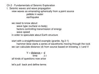
Ch 2 - Fundamentals of Seismic Exploration I. Seismic waves and wave propagation

1. Ch 2 - Fundamentals of Seismic Exploration • I. Seismic waves and wave propagation • view waves as emanating spherically from a point source • pebble in water • earthquake • we need to know about: • wave type (surface vs body) • factors controlling transmission of energy • wave speed • in order to speculate about Earth structure • start with a straightforward example (granite, fig 2-1) • hammer blow starts a series of wavefronts moving through the rock • we can calculate distance (d) from source based on knowing  t and V • V = distance = d • time  t • all kinds of questions now arise • let’s pull back and define terms

2. Wave terminology (Fig 2-2) • wavelength () = horiz distance of one wave cycle (eg, peak to peak or trough to trough) • amplitude (A)= vert dist from rest to max deflection of wave • period (T) = time it takes for passage of one cycle past a fixed point (like water waves passing a pier at Atlantic City (units often “seconds per cyle”) • frequency (f) = no. of cycles passing a pt per unit time (usu. “cycles per second” or “Hertz”) • easy to see relationships if you keep the units straight • frequency (f) = 1cycle • T seconds • V = distance x 1 cycle = distance • 1 cycle T seconds time • V =  x f • now assume path of propagation is  to wavefront; this is known as the “ray path”

3. Elastic Coefficients • now we start to focus on what controls speed of the wave • elastic relations between stress and strain are key - a force deforms a material, then it returns to original shape once stress is removed • think in terms of a wave instantaneously “loading” a rock, then rock immediately unloaded once wave crest is through • more terms to help describe the relations Y = mx + b  = E where E = slope = Young’s modulus of elasticity Stress,  Strain, 

4. Poisson’s ratio describes ratio of strain on x, y axes (fig 2-4) coincident with maximum and minimum compressive stress : •  = - 1 • 3 • Bulk modulus, K, relates volume change to external pressure, a way to describe its incompressibility (the higher the incompressibility, the less volume change occurs) • the shear or rigidity modulus, G, relates amt of sher deformation to amt of shear stress applied (the higher the rigidity, the less the material shears) • Note Table 2-1 -HOMEWORK - graph up these relationships…look for a pattern….what controls compressional wave velocity (Vp)?? • Look at  vs Vp • E vs Vp •  vs Vp • use the spreadsheet on disks in back of book if you like

5. Seismic Waves • 2 main types: • longitudinal - particle motion = compression/dilation like a slinky or spring, in direction of ray path travel- “p wave” for “primary” • transverse - particle motion = perpendic to direc of ray path travel, like shaking a rope - “s wave” for “secondary • p and s waves are body waves • Love and Rayleigh waves are surface waves (present only at surface) • Wave velocities • velocities controlled by 2 factors: density and elastic coefficients • for p waves, bulk mod, rigidity mod, and density control veloc • for s waves, rigidity mod and density control veloc • signif observations….. • Eq 2-13 demonstrates that p waves ALWAYS faster than s waves • s waves can’t travel through liquid

6. Some rules of thumb on p.18-19, table of velocities of materials saturated veloc>unsat (pore space filled) consol sed veloc>unconsol unwthrd rx veloc>wthrd unfrac rx veloc>frac think about these….why do these facts make sense? Note that velocities fall into broad groups but are non-unique: 500 m/sec - dry unconsolidated 1500 m/sec - wet unconsol 4000 m/sec for sed rx 6000 m/sec for ign rx return to looking at frequency, wavelength, veloc Veloc = dist =  x f time play with couple examples - given 1000 m/sec veloc, look at 2 diff seismic sources - 10 Hz, 100 Hz - what’s the wavelength of the signal in each of these cases?? Why is this important? Wavelength dictates vertical resolution, ability to “see”detail

7. II. Ray Paths in Layered Materials • key principles from both Huygen and Fermat • Huygen - fig 2-10 - all pts on spherical wavefront in turn become pt sources of spherical waves, new wavefront is a tangent line drawn along the new waves • Fermat - prin of least time….the wave (or ray) path between 2 pts is that path which takes least TIME to traverse (not the least distance) • in layer of const velocity, this will be the shortest straightline distance, but when you add diff layers, things may change…. • A. Reflection - • wave reflects any time it encounters a layer of diff velocity (lower or higher V) • terms important - know the angle of incidence (fig 2-11),   Raypath 

8. Now look at a reflection off the interface - what is it’s angle? • The same : angle incidence = angle of reflection • carry a step further - in terms of least time, what’s the path the reflected ray will take? Fig 2-12 • Burger derives the answer by using V = dist/time and a trig identity, sets up equation to show what is path of least time; path is where 1 = 2 • B. Refraction Fig 2-13 • equation to determine angle of refracted ray similar to that of reflected ray - result is relation known as Snell’s Law, VERY IMPORTANT • sin 1 = V1 • sin 2 V2 • (note that if velocity is same, like in reflec case, equa reduces to sin 1 = sin 2) • move to case of critical refraction angle - an important case • “critical angle” is angle of incidence required to generate a refraction….if incident ray is too shallow an angle, the ray will be totally reflected • Note that at the critical angle, the refracted ray runs in V2, parallel to the interface between layers V1 and V2 Fig 2-17

9. Equation for critical angle: •  = sin-1 (v1/v2) • why is this important? Figs 2-16 and 2-20 - the crit refracted wave is the one that will be taking the least time traveling through the lower layer, and it’s associated headwave will be the one that reaches the geophones first in actual field data collection • let’s pass on diffraction for now, move to…. • C. Wave arrivals at surface (see in Fig 2-20) • what do we expect to see? • P-wave arrival is what we’ll focus upon - it’s faster than shear wave, travels through more materials • but there are p waves arriving from several different routes… • air wave • direct wave • reflected wave • refracted (head) wave • to help visualize, look at table 2-4 …better yet, construct graph showing arrival time vs distance for these waves (FIG 2-21, 2-22) both show time vs distance…spend some time with this..lots of info here...

10. Tough to determine what signal is what at the first part of the seismic record… in gen, looks like the direct wave is the first to hit the geophones out to about 45 m, then the headwave is the fastest time 45 m source distance We’ll be coming back to this…for now, get the idea that diff p-wave paths exhibit diff velocities, and the “first arrival” at one geophone may not be from the same raypath as the first arrival at another geophone. Also, DO note that each straight line segment has a unique slope of time/distance….the inverse of velocity. This shows that these straight line segments represent ray paths with unique velocities.

11. III. Wave attenuation and amplitude • we want to discuss factors likely to alter wave amplitudes, because this helps our interpretations…. • We lose amplitude due to: • spherical spreading (table 2-5) • absorption (by material through which wave propagates) Table 2-6 • key here is to notice how much more energy is lost from high freqs than from low freqs… • we call the Earth a “low-pass” filter because it often transmits low freqs quite effectively, while blocking or filtering the highs • so you can see a problem in seis already - maintaining the high frequency content so the lows don’t overwhelm it • energy partitioning - an incident wave’s energy is broken up into reflected and refracted components(eg, Table 2-7) • couple rules of thumb here: • low incident angles (nearly ), most energy goes into refraction • high incident angles, most energy goes into reflection • this makes some intuitive sense…at high angles energy in wave is glancing off the reflector; when almost , energy can penetrate through the reflector • other factors controlling amplitude include original source strength, where located (above vs below surf), and coupling of both source and receiver to Earth

12. IV. Energy sources • depends upon land or sea, your needs, etc • Fig 2-26 shows energy & frequency spectra for familiar shallow sources • Vibroseis oscillatory sweeps provide good high freq signal but need lot of computer processing to generate seismograms • V. Seismic equipment - essentially focus on 3 areas: detecting the signal, conditioning or processing the signal from the detectors, recording the signal • A. detection- 2 types - seismometers or geophones - the job is the same • basic design is coil suspended in magnetic field; • when coil is moved in the field, an electric current and voltage is induced; • mvmt of coil and amt of voltage is proportional to the ground motion; • larger the ground motion, larger the signal • a complication arises with the natural resonant freq of a geophone- if excited to that freq, geophone will oscillate and distort the real incoming signal • some amt of damping is required to get a “flat response” - this means that geophone will respond equally to diff freqs Fig 2-30 • interesting pt made on geophone selection - we may want low freq, large amplitude first arrivals for refraction, but high freq for reflection

13. B. Signal conditioning (amplify & filter) • Amplify -typically want to suppress early strong signals, enhance later arrivals - some employ AGC (automatic gain control) which brings output amplitude at same level for all signals • Filter - cut out certain freqs, allow others to “pass” • filters help to cut out noise and to “restrict” the seis freqs recorded • with shallow reflection work, we want to maximize high freq response, so high-pass (low-cut) filters are used to pass through the highs but block the lows Figs 2-33 and 2-34 • C. Signal recording • big diff now vs yesteryear - digital vs analog • analog - waveform voltage recorded on rotating drum, like an eqk • looks fine but limitations exist in pulling out detail • digital - can convert analog signal to digital by sampling Fig 2-35 , increase your ability to pull out weak signals without distorting whole wave form • digital advantages are significant…direct read to computer, signal stacking that enhances signal-to-noise ratio, etc.