Download
1 / 12
130 likes | 599 Vues
High-Frequency Simulations of Global Seismic Wave Propagation. A seismology challenge: model the propagation of waves near 1 hz (1 sec period), the highest frequency signals that can propagate clear across the Earth.

E N D
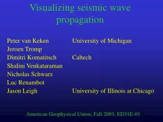
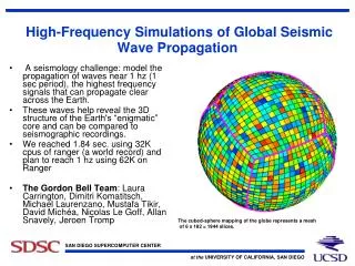
High-Frequency Simulations of Global Seismic Wave Propagation A seismology challenge: model the propagation of waves near 1 hz (1 sec period), the highest frequency signals that can propagate clear across the Earth. These waves help reveal the 3D structure of the Earth's “enigmatic” core and can be compared to seismographic recordings. We reached 1.84 sec. using 32K cpus of ranger (a world record) and plan to reach 1 hz using 62K on Ranger The Gordon Bell Team: Laura Carrington, Dimitri Komatitsch, Michael Laurenzano, Mustafa Tikir, David Michéa, Nicolas Le Goff, Allan Snavely, Jeroen Tromp The cubed-sphere mapping of the globe represents a mesh of 6 x 182 = 1944 slices.
1 slide summary SPECFEM3D_GLOBE is a spectral-element application enabling the simulation of global seismic wave propagation in 3D anelastic, anisotropic, rotating and self-gravitating Earth models at unprecedented resolution. A fundamental challenge in global seismology is to model the propagation of waves with periods between 1 and 2 seconds, the highest frequency signals that can propagate clear across the Earth. These waves help reveal the 3D structure of the Earth's deep interior and can be compared to seismographic recordings. We broke the 2 second barrier using the 32K processors of Ranger system at TACC reaching a period of 1.84 seconds with sustained 28.7 Tflops. We obtained similar results on the XT4 Franklin system at NERSC and the XT4 Kraken system at University of Tennessee Knoxville, while a similar run on the 28K processor Jaguar system at ORNL, which has more memory per processor, sustained 35.7 Tflops (a higher flops rate) with a 1.94 shortest period. This work is a finalist for the 2008 Gordon Bell Prize
A Spectral Element Method (SEM) Finite Earth model with volume Ω and free surface ∂Ω. An artificial absorbing boundary Γ is introduced if the physical model is for a “regional” model
For the purpose of computations, the Earth model Ω is subdivided into curved hexahedra whose shape is adapted to the edges of the model ∂Ω and Γ and to the main geological interfaces.
Weak form SEM Rather than using the equations of motion and associated boundary conditions directly: dotting the momentum equation with an arbitrary vector w, integrating by parts over the model volume Ω, and imposing the stress-free boundary condition where the stress tensor T is determined in terms of the displacement gradient s by Hooke's law The source term has been explicitly integrated using the the Dirac delta distribution
Meshing In the SEM mesh, grid points that lie on the sides, edges, or corners of an element are shared amongst neighboring elements, as illustrated. Therefore, the need arises to distinguish between the grid points that define an element, the local mesh, and all the grid points in the model, many of which are shared amongst several spectral elements, the global mesh.
Cubed sphere Split the globe into 6 chunks, each of which is further subdivided into n2 mesh slices for a total of 6 x n2 slices, The work for the mesher code is distributed to a parallel system by distributing the slices
Model guided sanity checking Performance model predicted that to reach 2 seconds 14 TB of data would have to be transferred between the mesher and the solver; at 1 second, over 108 TB So the two were merged
Improving locality To increase spatial and temporal locality for the global access of the points that are common to several elements, the order in which we access the elements can then be optimized. The goal is to find an order that minimizes the memory strides for the global arrays. We used the classical reverse Cuthill-McKee algorithm, which consists of renumbering the vertices of a graph to reduce the bandwidth of its adjacency matrix.
The relation between resolution and performance Resolution = 256*17 / Wave Period. (Higher resolution is higher frequency).
Results Simulation of an earthquake in Argentina was run successively on 9,600 cores (12.1 Tflops sustained), 12,696 cores (16.0 Tflops sustained), and then 17,496 cores of NICS’s Kraken system. The 17K core run sustained 22.4 Tflops and had a seismic period length of 2.52 seconds; temporarily a new resolution record. On the Jaguar system at ORNL we simulated the same event and achieved a seismic period length of 1.94 seconds and a sustained 35.7 Tflops (our current flops record) using 29K cores. On the Ranger system at TACC the same event achieved a seismic period length 1.84 seconds (our current resolution record) with sustained 28.7 Tflops using 32K cores.