First topic: clustering and pattern recognition
First topic: clustering and pattern recognition. Marc Sobel. Examples of Patterns. Pattern discovery and association. Statistics show connections between the shape of one’s face (adults) and his/her Character. There is also evidence that the outline of children’s

First topic: clustering and pattern recognition
E N D
Presentation Transcript
Examples of Patterns Pattern discovery and association Statistics show connections between the shape of one’s face (adults) and his/her Character. There is also evidence that the outline of children’s face is related to alcohol abuse during pregnancy.
Examples of Patterns Crystal patterns at atomic and molecular levels Their structures are represented by 3D graphs and can be described by deterministic grammar or formal language
Examples of Patterns with clusters Patterns of brain activities: We may understand patterns of brain activity and find relationships between brain activities, cognition, and behaviors
What is a pattern? (see Grenander for a full theory) In plain language, a pattern is a set of instances which share some regularities, and are similar to each other in the set. A pattern should occur repeatedly. A pattern is observable, sometimes partially, by some sensors with noise and distortions. How do we define “regularity”? How do we define “similarity”? How do we define “likelihood” for the repetition of a pattern? How do we model the sensors? One feature of patterns is that they result from similar groups of data called clusters. How can we identify these clusters.
Hard K-means algorithm (Greedy) • Start with points x1,…,xn to be clustered. and mean (cluster) centers m1[0],…,mk[0] (at time t=0). Iterate the following steps: 1) Assign x’s to the means according to their minimum distance from them. Let Zi=l iff xi gets assigned to class l. (i=1,…,n; l=1,…,k). 2) Update the means according to:
Greedy versus nongreedy algorithms • Greedy algorithms optimize an objective function at each step. The objective function for the k-means algorithm is: • Where ‘mj[i]’ means the nearest cluster center to the point xi (i=1,…,n). • Greedy algorithms are useful but (without external support) are subject to many problems like overfitting, selecting ‘local’ in place of global optima, etc…
Problems with hard k-means • 1. Convergence depends on starting point. • 2. k-means is a hard assignment algorithm which means that both important points and outliers play a similar role in assignment. • 3. Components with different sizes induce a strong bias on the classification • 4. The distance used plays an enormous role in the kind of clusters which result (e.g., if we used minikowski distance, d(xi,xj)=║xi-xl║α(alpha has an effect) ---possible project.
Soft k-means Version 1: An improvement? • In soft k-means, we assign points to clusters with certain probabilities or weights rather than in the usual hard manner: • For parameters β either known, estimated prior to implementation, or iteratively estimated.
Soft k means • We update the means by the update: • (j=1,..,k). • This way, points which are between clusters get assigned to ‘both of them’ and hence play a dual role.
Soft k-means Version 1 (continued) • Typically, the parameter β (called the stiffness) plays a significant role. If β goes to infinity, the algorithm tends to that of hard k means. If β tends to 0, the algorithm tends to assign points randomly to clusters. If β tends to minus infinity, the algorithm assigns points to clusters far away from themselves. (Possible Project)
Stiffness Assignment • Typically, because β is an information type parameter – the bigger it is, the more information used about the points -- and since (1/σ2) also measures the amount of information the data are providing, we assign β= (1/σ2) . Possible Project: What impact does the use of different stiffness parameters have on clustering a particular data set.
The effects of using a stiffness for different values of β when it is assigned it’s ‘information’ value
Possible Projects • 1. What happens to the clusters (under soft clustering version 1) with information assignment) when we start with data which is a mixture of two gaussians. Mixtures of gaussians just means that, with a certain probability, data is one gaussian and with one minus that probability, it is another gaussian. • 2. What happens to the clusters when we have data which consists of two independent gaussians.
Gaussian Distributions • Gaussian Distributions: One-dimensional Gaussian distributions: m is the mean and σ is the standard deviation. Multidimensional Gaussian distribution:
Independent Gaussians • In the case of independent spherical Gaussians with common sigma:
Soft k-means Version 2 • In soft k-means version 2, we assign different stiffness values and different proportions to each separate cluster: We now use the notation sigma instead of β.
Similarity of soft k-means with EM algorithm • Now assume a data set consisting of gaussian variables x1,…,xn with means among the set {m1,…,mk } and standard deviations in the set {σ1,…,σk}. We write the log likelihood as: • Maximum likelihood estimators maximize this over the parameters. We just differentiate with respect to each mu and sigma and set to 0.
EM algorithm continued • The critical equations for the mu’s and sigma’s are: • But, we don’t know what the Z’s are. Therefore, we substitute estimates for them: • In place of a hard assignment, we substitute the probabilities:
Bayes Rule • Above, we have used Bayes rule: • For events A1,…,Ad whose probabilities sum to 1; and events B:
Bayes Rule for Discrete variables • For random variables, Bayes rule becomes: • For a discrete random variable X, Y:
Bayes Rule for Continuous variables • For random variables, Bayes rule becomes: • For a continuous random variable X, Y:
EM (recontinued) • Finally, we substitute πf for the probability • P(Zi=f) (i=1,…,n; f=1,…,k). This adds additional parameters which can be updated via: • This is the assignment step in the soft k-means algorithm --- in EM it is called the E step.
EM algorithm concluded • Substituting we get: • This is the update step in the soft k-means algorithm. In EM it is called the M step.
Assuming a single stiffness parameter • We get, • Now, a little bit of algebra shows that we are back at the soft means formulation: σ2=(1/β)
Does EM work? • As presented above: no!!!!!!!!!!! • The problem is typically that: • 1. assuming a single stiffness (sd) means that we will not properly capture large/small components. • 2. assuming multiple standard deviations, the resulting sigma’s get mis-estimated because they are very sensitive to mis-estimating the component means.
Possible Projects • Show by simulating a mixture distribution with small and large component that both the soft k-means versions 1 and 2 fail to work under certain settings. (Hint: suppose you put ‘m’ = an isolated point). • What happens if you have ‘non-aligned’ components (i.e., they are stretched at a different angle from the other components). What will the EM algorithm described above do?

