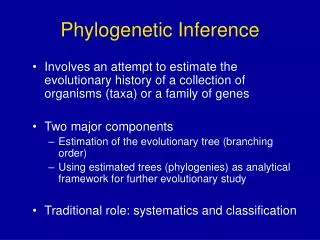
Phylogenetic inference
Bioinformatics. Phylogenetic inference. Structure of phylogenetic trees. A. F. H. B. C. G. I. D. Root. E. Evolutionary relationships between objects of studies (organisms, organs, sequences) are represented by phylogenetic trees.

Phylogenetic inference
E N D
Presentation Transcript
Bioinformatics Phylogenetic inference
Structure of phylogenetic trees A F H B C G I D Root E • Evolutionary relationships between objects of studies (organisms, organs, sequences) are represented by phylogenetic trees. • Trees are particular types of graphs made of nodes and branches • Nodes = taxonomic units • Leaves = Operational Taxonomic Units (OTU): extant species (ex: A, B, C, D, E) • Internal nodes = Hypothetical taxonomic units = HTU: ancestral species (F, G, H, I). • Branches = kin relationship (ancestry, descendence) between taxonomic units. • Internal branches • External branches • The set of branching of a tree is called topology • Source: Emese Meglézc
Rooted versus non-rooted trees A F H B C B C G D H G I F A I Racine D E E • The root defines a unique evolutionary path towards each leave. • It represents the last common ancestor (i.e. the most recent one) of all the OTU. • Non-rooted trees are not properly speaking phylogenetic, since they have no temporal direction -> do not indicate the type of relationship (ancestor, descendent, cousin, …) between nodes. Arbre enraciné Arbre non-enraciné
How to root a phylogenetic tree ? Loup F H Chien Souris Loup Souris G Rat H G I F Chien I Racine Rat Poulet Poulet • « Outgroup »: if the OTU of interest include an outgroup (a group very distant from all the other ones), one can enroot the tree on its branch. • Example: dog, wolf, mouse, rat and chicken • Based on our prior biological knowledge, we decide that the outgroup is chicken. • In absence of a prior knowledge on the outgroup: • Mean weight rooting: the tree is rooted on the branch which minimises the mean distance to the leaves. • This assumes a molecular clock: mutation rates are supposed to be constant during evolution, and similar along all the branches of the tree. • This hypothesis is generally not valid, it is only an approximation. • Adapté d’après Emese Meglézc
Isomorphisms of phylogenetic trees B C F G H H D A B C G F I I Racine Racine D A E E • One should avoid the trap consisting in evaluating distances between leaves on the basis of their vertical proximity on a tree drawing. • The two structures below are topologically absolutely identical. • However, leaves B and D seem close on the left graph, and distant on the right graph. • To evaluate the distance between two nodes of a tree, one must take into account the total length of the shortest path between them (sum of branch lengths). • Source: Emese Meglézc
Scale of a phylogenetic tree A F H B C G I Racine D E • Representation with scale • This tree represents the evolutionary distances between nodes. • Branch lengths are proportional to the number of evolutionary events (substitutions or substitutions/sites). • Scale-less representation • The tree only represents the branching order. • Branch lengths are not proportional to the number of evolutionary changes. A F B H C G I Racine D E 0,1 • Source: Emese Meglézc
Cladistics, cladograms and clades • Cladistics • (Greek: klados = branch) is a branch of biology that determines the evolutionary relationships between organisms based on derived similarities (source: Wilkipaedia). • Cladogram • tree-like drawing, usually with binary bifurcations, representing one evolutionary scenario about divergences between species or sequences. • Clade • Any sub-tree of a cladogram. • Note • Branch lengths to not reflect evolutionary time. • The cladogram only represents branching successions, not the time.
Cladistics, cladograms and clades • This is also a cladogram • Although branches are rectangular, the drawing only represents the succession of evolutionary events, without attempt to display any time scale.
Phylogram • Phylogram : branch lengths represent the number of evolutionary events (mutations, changes); • The phylogram shown here represents the inferred phylogeny of Mammalian opsins. The root should be placed between the groups SW (short-wave-sensitive) and LW+MW (Long-+medium-wave-sensitive). • Notes: • the relative scale is at the bottom. • this tree is unrooted, despite the fact that it is displayed in a left-to-right orientation; • the distance between two nodes is the sum of segment lengths to join them; • the vertical distance can thus be misleading: two successive leaves on the vertical axis (e.g. LW Tachyglossus and SW mouse) can nevertheless be very distant when following the branches; • lengths are only approximations of the inferred distances;
Molecular clock • Chronogram: branch lengths represent evolutionary time. • The "molecular clock" hypothesis (left tree) assumes that rates of evolution do not vary between branches. All leaf nodes are thus aligned vertically, since they represent contemporaneous species. • This hypothesis is not always valid: in some cases, two genes can diverge from a common ancestor, but one of them may have diverged faster than the other one. • This is a rather classical mechanism of evolution: a duplication creates some redundancy, and one copy of the gene will evolve whereas the other one retains the initial function (and mutations are counter-selected). Ultrametric tree (with clock) (e.g. UPGMA) Without clock (e.g. neighbour-joining)
Summary – tree-based representations • Didier Casane & Patrick Laurenti (2012). Penser la biologie dans un cadre phylogénétique: l’exemple de l’évolution des vertébrés. Médecine/Sciences.
Species trees versus molecule tree • A species tree aims at representing the evolutionary relationships between species. • A molecule tree represents the evolutionary history of a family of related molecules (genes, proteins). • Species trees and molecule trees are generally related ... • Species tree can be inferred from various criteria, including the history of carefully chosen molecules. • ... but not identical. • A molecular family can contain several copies in the same species (in-paralogs), due to gene duplications. • Some molecules can be transferred horizontally between species. • Due to combinations of duplications/divergences/deletions, the tree of a given gene may be inconsistent with the species tree. • Illustration: Figure 7.3 from Zvelebil and Baum. Source: Zvelebil, M.J. and Baum, J.O. (2008) Understanding Bioinformatics. Garland Science, New York and London.
Reconciliation between molecular and species trees Source: Zvelebil, M.J. and Baum, J.O. (2008) Understanding Bioinformatics. Garland Science, New York and London.
Concept definitions from Fitch (2000) • Discussion about definitions of the paper • Fitch, W. M. (2000). Homology a personal view on some of the problems. Trends Genet 16, 227-31. • Homology • Owen (1843). « the same organ under every variety of form and function ». • Fitch (2000). Homology is the relationship of any two characters that have descendent, usually with divergence, from a common ancestral character. • Note: “character” can be a phenotypic trait, or a site at a given position of a protein, or a whole gene, ... • Molecular application: two genes are homologous if diverge from a common ancestral gene. • Analogy: relationship of two characters that have developed convergently from unrelated ancestors. • Cenancestor: the most recent common ancestor of the taxa under consideration • Orthology: relationship of any two homologous characters whose common ancestor lies in the cenancestor of the taxa from which the two sequences were obtained. • Paralogy: Relationship of two characters arising from a duplication of the gene for that character. • Xenology: relationship of any two characters whose history, since their common ancestor, involves interspecies (horizontal) transfer of the genetic material for at least one of those characters. • Analogy • Homology • Paralogy • Xenology or not (xeonologs from paralogs) • Orthology • Xenology or not • (xeonologs from orthologs)
Exercise • On the basis of Zvelebil & Baum’s definitions (below), qualify the relationships between each pair of genes in the illustrative schema. • P paralog • O ortholog • X xenolog • A analog • Orthologs can fomally be defined as a pair of genes whose last common ancestor occurred immediately before a speciation event (ex: a1 and a2). • Paralogs can fomally be defined as a pair of genes whose last common ancestor occurred immediately before a gene duplication event (ex: b2 and b2'). Source: Zvelebil & Baum, 2000
Exercise • Example: B1 versus C1 • The two sequences (B1 and C1) were obtained from taxa B and C, respectively. • The cenancestor (blue arrow) is the taxon that preceded the second speciation event (Sp2). • The common ancestor gene (green dot) coincides with the cenancestor • -> B1 and C1 are orthologs • Orthologs can fomally be defined as a pair of genes whose last common ancestor occurred immediately before a speciation event. • Paralogs can fomally be defined as a pair of genes whose last common ancestor occurred immediately before a gene duplication event. • Source: Zvelebil & Baum, 2000
Exercise • Example: B1 versus C2 • The two sequences (B1 and C2) were obtained from taxa B and C, respectively. • The common ancestor gene (green dot) is the gene that just preceded the duplication Dp1. • This common ancestor is much anterior to the coenancestor between the two species (blue arrow). • -> B1 and C2 are paralogs • Orthologs can fomally be defined as a pair of genes whose last common ancestor occurred immediately before a speciation event. • Paralogs can fomally be defined as a pair of genes whose last common ancestor occurred immediately before a gene duplication event. • Source: Zvelebil & Baum, 2000
Solution to the exercise • On the basis of Zvelebil & Baum’s definitions (below), qualify the relationships between each pair of genes in the illustrative schema. • P paralog • O ortholog • X xenolog • A analog • Orthologs can fomally be defined as a pair of genes whose last common ancestor occurred immediately before a speciation event (ex: a1 and a2). • Paralogs can fomally be defined as a pair of genes whose last common ancestor occurred immediately before a gene duplication event (ex: b2 and b2'). Source: Zvelebil & Baum, 2000
Reconciliation between species and molecular trees A1 AB1 B1 C1 B2 C2 C3 A, B, C represent species Speciation Duplication
How many trees ? • The number of possible trees increases drastically with the number of terminal elements (leaves, which can represent molecules or species). • Only one of those trees corresponds to the real evolutionary history. • Since we do not dispose of this tree a priori, it must be inferred from the current elements (the operational taxonomic units, OTU).
Characters and character states • Character: feature (quantitative or qualitative) that can be observed in an organism. • State of a character: particular form of a character in a particular OTU (continuous or discrete variable). • Examples • Character: size of left posterior leg. Character state: 1.68cm. • Character: aminoacid at position 68 of the protein encoded by the gene CYTB. Character state: alanine.
Example: opsins • To infer a phylogenetic tree for a family of sequences, we start from a multiple alignment. • The figure below shows the first half of a multiple alignment between 50 Mammalian opsins. • By simple visual inspection, we already distinguish 2 obvious groups: • Top : long- (LW) and medium-wave-sensitive (MW) opsins • Bottom: short-wave-sensitive (SW) opsins
Methods for inferring a phylogenetic tree • Cladistic methods • Based on the study of characters (nucleotides, aminoacids, presence/absence of a deletion/insertion, …) • Maximum of parsimony. • Distance-based methods • Based on distance measurements (ex: number of substitutions per site). • UPGMA, Neighbour-Joining (NJ), evolutionary minimum, least squares, … • Statistical methods • Based on a study of the states of characters + on distances • Maximum likelihood • Bayesian methods
Phylogenetic inference from sequence comparison • Alternative approaches • Maximum parsimony • Distance • Maximum likelihood Unaligned sequences Sequence alignment Aligned sequences strong similarity ? many (> 20) sequences ? Maximum parsinomy yes no Source: Mount (2000)
Parsimony method • Principle: • Identify the topoloy (T) involving the smallest umber of evolutionary changes, which is sufficient to account for observed differences between studied OTUs. • Based on discrete characters => the most parcimonious tree correspond to the shortest path (in terms of changes) leading to the observed character states. • Algorithm • Build all possible trees • For each site (position in the alignment), count the minimal number of substitutions explaining this tree • Retain the tree requiring the smallest total number of substitutions (taking all sites into account). • Features of the trees • Multiple solutions can be found : several trees with the same minimal number of changes • Branch lengths do not indicate the evolutionary distance (scale-less tree) • Unrooted trees.
Matrice de caractères Sites Séquences
Maximum de parcimonie - Méthode Déterminer toutes les topologies possibles 4 UTO => 3 arbres non racinés
A A A C B B D D C B C D Maximum de parcimonie - Méthode Déterminer toutes les topologies possibles 4 UTO => 3 arbres non racinés
A A A C B B A A A A A A A A A A A A C D D D C B Maximum de parcimonie - Méthode Étude du caractère n°1 Caractère constant (même état de caractère à tous les sites) Caractère ne favorisant aucune topologie par rapport à une autre Nb CE= 0 Nb CE= 0 Nb CE= 0
A A A C B B A A A G G G G G G G G G C D D D C B Maximum de parcimonie - Méthode Étude du caractère n°2 Caractère variable mais non informatif Caractère ne favorisant aucune topologie par rapport à une autre Nb CE= 1 Nb CE= 1 Nb CE= 1
A A A C B B G G G C C A C A A A A A D D C D C B Maximum de parcimonie - Méthode Étude du caractère n°3
A A A A A C B C C B G G G A C C C A A A A A D D C D D C B B D B Maximum de parcimonie - Méthode Étude du caractère n°3 G A C A Arbre 1 G A C A Nb CE= 2
A A A C B B G G G C A C C A A A A A C D D D C B Maximum de parcimonie - Méthode Étude du caractère n°3 Caractère variable mais non informatif Caractère ne favorisant aucune topologie par rapport à une autre Nb CE= 2 Nb CE= 2 Nb CE= 2
A A A C B B A A A C T C C T G G G T C D D D C B Maximum de parcimonie - Méthode Étude du caractère n°4 Caractère variable mais non informatif Caractère ne favorisant aucune topologie par rapport à une autre Nb CE= 3 Nb CE= 3 Nb CE= 3
A A A C B B D D C B C D Maximum de parcimonie - Méthode Étude du caractère n°5 Nb CE= ? Nb CE= ? Nb CE= ?
A A A C B B G G G G A G G A A A A A C D D D C B Maximum de parcimonie - Méthode Étude du caractère n°5 Caractère variable et informatif (au moins 2 états de caractère sont partagés par au moins 2 OTU) Caractère favorisant la première topologie par rapport aux deux autres Nb CE= 1 Nb CE= 2 Nb CE= 2
Maximum parsimony Column 5 mutation seq1 G A seq3 G A seq2 G A seq4 seq 1G G seq 2 A A seq 3 A A seq 4 seq 1G G seq 2 A A seq 4 A A seq 3 • For each column of the alignment, all possible trees are evaluated and the tree with the smallest number of mutations is retained • The trees which fit with the highest number of columns are retained • The program can return several trees Adapted from Mount (2000)
A A A C B B T T T T T T T T T T T T C D D D C B Maximum de parcimonie - Méthode Étude du caractère n°6 Caractère constant (même état de caractère chez tous les OTUs) Caractère ne favorisant aucune topologie par rapport à une autre Nb CE= 0 Nb CE= 0 Nb CE= 0
A A A C B B T T T T C T T C C C C C C D D D C B Maximum de parcimonie - Méthode Étude du caractère n°7 Caractère variable et informatif Caractère favorisant la première topologie par rapport aux deux autres Nb CE= 1 Nb CE= 2 Nb CE= 2
A A A C B B C C C C C C C C C C C C C D D D C B Maximum de parcimonie - Méthode Étude du caractère n°8 Caractère constant (même état de caractère à tous les OTUs) Caractère ne favorisant aucune topologie par rapport à une autre Nb CE= 0 Nb CE= 0 Nb CE= 0
A A A C B B D D C B C D Maximum de parcimonie - Méthode Étude du caractère n°9 Nb CE= ? Nb CE= ? Nb CE= ?
A A A C B B A A A T A T T A T T T A C D D D C B Maximum de parcimonie - Méthode Étude du caractère n°9 Caractère variable et informatif Caractère favorisant la deuxième topologie par rapport aux deux autres Nb CE= 2 Nb CE= 1 Nb CE= 2
A A A C B B D D C B C D Maximum de parcimonie - Méthode Bilan: T1 = 0+1+2+3+1+0+1+0+2=10 T2 = 0+1+2+3+2+0+2+0+1=11 T3 = 0+1+2+3+2+0+2+0+2=12 L’arbre le plus parcimonieux = arbre 1 Nb CE= 10 Nb CE= 11 Nb CE= 12
Maximum de parcimonie – classification des sites • Caractères invariants si toutes les OTU possèdent le même état de caractères pour un site donné • Caractères variables • Non informatif si les états de caractères à ce site ne favorisent aucune topologie parmi l’ensemble des topologies possibles • Informatif si les états de caractères à ce site favorise une (ou plusieurs) topologie(s) parmi l’ensemble des topologies possibles
Maximum parsimony example • Parsimony tree calculated from a multiple alignment of the E.coli proteins containing a lacI-type HTH domain • Scale-less unrooted tree • Left: text representation (protpars output) • Bottom right: visualized with njplot (in the ClustalX distribution) +-----------CYTR_ECOLI +--------------------------6 ! ! +--------EBGR_ECOLI ! +-13 ! ! +-----CSCR_ECOLI ! +-12 ! ! +--IDNR_ECOLI ! +--5 ! +--GNTR_ECOLI +--4 ! ! +-----MALI_ECOLI ! ! +-10 ! ! ! ! +--TRER_ECOLI ! ! +--------------9 +-14 ! ! ! ! +--YCJW_ECOLI ! ! ! ! ! ! ! +--------LACI_ECOLI ! +--------------8 +--2 ! +--FRUR_ECOLI ! ! ! +-------15 ! ! ! ! +--RAFR_ECOLI ! ! +----------11 ! ! ! +-----ASCG_ECOLI ! ! +-----7 --1 ! ! +--GALS_ECOLI ! ! +--3 ! ! +--GALR_ECOLI ! ! ! +-----------------------------------------RBSR_ECOLI ! +--------------------------------------------PURR_ECOLI remember: this is an unrooted tree! requires a total of 4095.000
Maximum of parsimony – drawbacks of the method • The number of possible trees increases rapidly with the number of UTOs (sequences). • In the preceding example we analyzed 4 sequences only. • For 20 sequences, we would need to treat an astronomical number of possibilities. • Parsimony intrinsically relies on an assumption of molecular clock -> assumes that all the branches evolved at the same speed. • This method only works with highly conserved sequences.
Phylogenetic inference from sequence comparison • Alternative approaches • Maximum parsimony • Distance • Maximum likelihood • Source: Mount (2000) Unaligned sequences Sequence alignment Aligned sequences strong similarity ? many (> 20) sequences ? Maximum parsinomy yes no no yes clear similarity ? Distance yes
Distance method • Starting from a multiple alignment, calculate the distance between each pair of sequences • Calculate a tree which fits as well as possible with the distance matrix • branch lengths should correspond to distances • rooted or unrooted • Several methods can be used for calculating a tree from the distance matrix. • Fitch-Margoliah • Neighbour-Joining • UPGMA Aligned sequences Distance calculation Distance matrix Tree calculation Tree