Download
1 / 18
210 likes | 279 Vues
Explore the goals, assumptions, and processes of phylogenetic analysis, including sequence selection, alignment construction, distance calculation, tree building, and evaluation methods. Learn about pair-wise distances, tree construction steps, and tree evaluation techniques like bootstrapping.

E N D
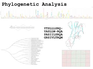
BI420 – Introduction to Bioinformatics Phylogenetic Analysis Gabor T. Marth Department of Biology, Boston College marth@bc.edu Figures from Higgs & Attwood
The goals of phylogenetics To understand the evolutionary relationships among species, e.g. - the order in which they diverged - the time since divergence
The assumptions in phylogenetics • Any group of organisms are related to each other by descent from a common ancestor • The relationships between organisms are described by a bifurcating tree • Change in characteristics between organisms occurs over time
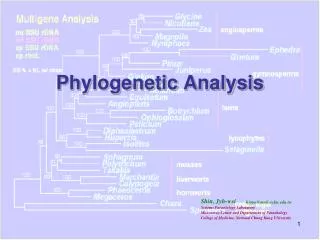
Phylogenetic “objects” Phylogenetic tree node branch taxon clade
Constructing an evolutionary tree Step 1. Selection of appropriate sequences Step 2. Construction of multiple sequence alignment Step 3. Calculation of pair-wise evolutionary distances Step 4. Tree construction Step 5. Tree evaluation
1. Sequence selection • find sequences with an appropriate amount of divergence: there can be too little or too much divergence (e.g. genes identical across taxa, or non-conserved genomic sequence) • try to select orthologous sequences to make sure that the genes used for tree construction are likely to have preserved functions
2. Multiple alignment (mitochondrial small subunit RNA gene) • informative sites • alignment editing • mechanics of multiple alignment construction covered in earlier classes in the course
3. Pair-wise distance • measures how diverged two sequences are: ACGCGTTATTACAGTTGACT ACACGTTATGACAGTTGACT 2 differences in 20bp D = 2/20 = 0.1 (10% divergence) • how evolutionarily distant two sequences are: Jukes-Cantor (JC) d = -3/4 ln(1-D*4/3) = 0.10732 (evolutionary distance)
Pair-wise distances Pair-wise JC distance matrix
More complex substitution models • substitutions between less similar residues indicate more divergence than between more similar residues (hydrophobic vs. hydrophilic) A C G T A - 2 1 2 C 2 - 2 1 G 1 2 - 2 T 2 1 2 - ACGCGTTATTACAGTTGACT ACACGTTATGACAGTTGACT A/G (1) + T/G (2) diff = 3 • amino acid substitution matrices (e.g. PAM, BLOSUM)
4. Tree construction • goal is to group (cluster) sequences in a hierarchical fashion • each step creates a “node” that represents the common ancestor of all the species/sequences within the group CA of group containing (A,B,C,D) CA of group containing (A,B) CA of group containing (A,B)
UPGMA method for phylogeny construction UPGMA (unweighted pair-group method with arithmetic mean) is conceptually very simple Step #1. Cluster two nodes with the shortest distance: e.g. if d(C,D) is lower than d(A,B), d(A,C), etc. then group C and D together. CD is now a new “node” Step #2. re-calculate distance between new node CD and all other current node, e.g.: d(CD, A) = ½ * (d(C,A) + d(D,A)) CD Go to Step #1. until every node is clustered into a single group
Example UPGMA phylogeny from a given distance matrix First cluster: Chimp + Pygmy chimp
Example (cont’d) After performing the complete clustering with UPGMA, we get the following rooted tree: There are many other tree-building methods (see Higgs & Attwood)
Branch lengths ultra-metricity additivity
Rooted vs. un-rooted trees Tree rooted with an outgroup (rodents)
5. Tree evaluation • Goal: to evaluate the strength of the phylogenetic signal in the data and the robustness of the tree • Bootstrapping: re-sample the original columns of the alignment with replacement, and produce a random, artificial alignment
Bootstrap support • Report: for each node, the %-age of times resampled alignments produced the same tree topology (from that node down to the leaves) weak bootstrap support strong bootstrap support