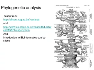
Evolutionary Context in Bioinformatics Analysis
Explore the theory of evolution, phylogenetic reconstruction methods, and molecular data applications in bioinformatics analysis. Understand terminology, classification, and the basis of systematics. Discover how to interpret phylogenetic trees and use molecular data effectively.

Evolutionary Context in Bioinformatics Analysis
E N D
Presentation Transcript
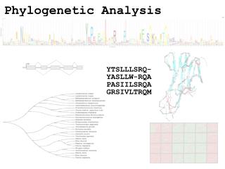
Phylogenetic AnalysisUnit 16 BIOL221T: Advanced Bioinformatics for Biotechnology Irene Gabashvili, PhD
B&O, chapter 14 • Bioinformatics analyses should be interpreted in evolutionary context • Good-quality sequence alignments important for evolutionary analysis • Common phylogenetic methods and software are different – be cautious when using and interpreting your results
Terminology and the Basics • Phylogenetics is sometimes called claudistics • Clade – a set of descendants from a single ancestor (greek for branch). • 3 basic assumptions: • Any group of organism descended from a common ancestor • Bifurcating pattern of cladogenesis • Change in characteristics occurs in lineages over time
Classification: Linnaeus Carl Linnaeus 1707-1778
Classification: Linnaeus • Hierarchical system • Kingdom (Rige) • Phylum (Række) • Class (Klasse) • Order (Orden) • Family (Familie) • Genus (Slægt) • Species (Art)
Classification depicted as a tree Species Genus Family Order Class
Theory of evolution Charles Darwin 1809-1882
Phylogenetic basis of systematics • Linnaeus: Ordering principle is God. • Darwin: Ordering principle is shared descent from common ancestors. • Today, systematics is explicitly based on phylogeny.
Darwin’s four postulates • More young are produced each generation than can survive to reproduce. • Individuals in a population vary in their characteristics. • Some differences among individuals are based on genetic differences. • Individuals with favorable characteristics have higher rates of survival and reproduction. • Evolution by means of natural selection • Presence of ”design-like” features in organisms: quite often features are there “for a reason”
Theory of evolution as the basis of biological understanding ”Nothing in biology makes sense, except in the light of evolution. Without that light it becomes a pile of sundry facts - some of them interesting or curious but making no meaningful picture as a whole” T. Dobzhansky
Terminology • Clades – monophyletic taxon • Taxons – any named group of organism • Branches – divergence (length may indicate the degree) • Nodes – any bifurcating branch point
Trees: representations Three different representations of the same tree
Trees: rooted vs. unrooted • A rooted tree has a single node (the root) that represents a point in time that is earlier than any other node in the tree. • A rooted tree has directionality (nodes can be ordered in terms of “earlier” or “later”). • In the rooted tree, distance between two nodes is represented along the time-axis only (the second axis just helps spread out the leafs) Early Late
Trees: rooted vs. unrooted • A rooted tree has a single node (the root) that represents a point in time that is earlier than any other node in the tree. • A rooted tree has directionality (nodes can be ordered in terms of “earlier” or “later”). • In the rooted tree, distance between two nodes is represented along the time-axis only (the second axis just helps spread out the leafs) Early Late
Trees: rooted vs. unrooted • A rooted tree has a single node (the root) that represents a point in time that is earlier than any other node in the tree. • A rooted tree has directionality (nodes can be ordered in terms of “earlier” or “later”). • In the rooted tree, distance between two nodes is represented along the time-axis only (the second axis just helps spread out the leafs) Early Late
Trees: rooted vs. unrooted • In unrooted trees there is no directionality: we do not know if a node is earlier or later than another node • Distance along branches directly represents node distance
Trees: rooted vs. unrooted • In unrooted trees there is no directionality: we do not know if a node is earlier or later than another node • Distance along branches directly represents node distance
Data: molecular phylogeny • DNA sequences • genomic DNA • mitochondrial DNA • chloroplast DNA • Protein sequences • Restriction site polymorphisms • DNA/DNA hybridization • Immunological cross-reaction
Morphology vs. molecular data African white-backed vulture (old world vulture) Andean condor (new world vulture) New and old world vultures seem to be closely related based on morphology. Molecular data indicates that old world vultures are related to birds of prey (falcons, hawks, etc.) while new world vultures are more closely related to storks Similar features presumably the result of convergent evolution
Molecular data: single-celled organisms Molecular data useful for analyzing single-celled organisms (which have only few prominent morphological features).
Distance Matrix Methods • Construct multiple alignment of sequences • Construct table listing all pairwise differences (distance matrix) • Construct tree from pairwise distances Gorilla : ACGTCGTA Human : ACGTTCCT Chimpanzee: ACGTTTCG Ch 1 1 1 Hu 2 Go
Finding Optimal Branch Lengths S2 S1 a c b e d S3 S4 Distance along tree Observed distance D12 d12 = a + b + c D13 d13 = a + d D14 d14 = a + b + e D23 d23 = d + b + c D24 d24 = c + e D34 d34 = d + b + e Goal:
Optimal Branch Lengths: Least Squares • Fit between given tree and observed distances can be expressed as “sum of squared differences”: Q = (Dij - dij)2 • Find branch lengths that minimize Q - this is the optimal set of branch lengths for this tree. S2 S1 a c b e d S3 S4 Distance along tree j>i D12 d12 = a + b + c D13 d13 = a + d D14 d14 = a + b + e D23 d23 = d + b + c D24 d24 = c + e D34 d34 = d + b + e Goal:
Least Squares Optimality Criterion • Search through all (or many) tree topologies • For each investigated tree, find best branch lengths using least squares criterion • Among all investigated trees, the best tree is the one with the smallest sum of squared errors.
Heuristic search • Construct initial tree; determine sum of squares • Construct set of “neighboring trees” by making small rearrangements of initial tree; determine sum of squares for each neighbor • If any of the neighboring trees are better than the initial tree, then select it/them and use as starting point for new round of rearrangements. (Possibly several neighbors are equally good) • Repeat steps 2+3 until you have found a tree that is better than all of its neighbors. • This tree is a “local optimum” (not necessarily a global optimum!)
Clustering Algorithms • Starting point: Distance matrix • Cluster least different pair of sequences: • Tree: pair connected to common ancestral node, compute branch lengths from ancestral node to both descendants • Distance matrix: combine two entries into one. Compute new distance matrix, by finding distance from new node to all other nodes • Repeat until all nodes are linked • Results in only one tree, there is no measure of tree-goodness.
Neighbor Joining Algorithm • For each tip compute ui = jDij/(n-2) (this is essentially the average distance to all other tips, except the denominator is n-2 instead of n) • Find the pair of tips, i and j, where Dij-ui-uj is smallest • Connect the tips i and j, forming a new ancestral node. The branch lengths from the ancestral node to i and j are: vi = 0.5 Dij + 0.5 (ui-uj) vj = 0.5 Dij + 0.5 (uj-ui) • Update the distance matrix: Compute distance between new node and each remaining tip as follows: Dij,k = (Dik+Djk-Dij)/2 • Replace tips i and j by the new node which is now treated as a tip • Repeat until only two nodes remain.
Superimposed Substitutions • Actual number of evolutionary events: 5 • Observed number of differences: 2 • Distance is (almost) always underestimated ACGGTGC C T GCGGTGA
Model-based correction for superimposed substitutions • Goal: try to infer the real number of evolutionary events (the real distance) based on • Observed data (sequence alignment) • A model of how evolution occurs
Jukes and Cantor Model • Four nucleotides assumed to be equally frequent (f=0.25) • All 12 substitution rates assumed to be equal • Under this model the corrected distance is: DJC = -0.75 x ln(1-1.33 x DOBS) • For instance: DOBS=0.43 => DJC=0.64
Homologs • Orthologs - speciation • Paralogs - duplication • Xenologs – horizontal transfer
Clustering Algorithms Clustering algorithms use distances to calculate phylogenetic trees. These trees are based solely on the relative numbers of similarities and differences between a set of sequences. • Start with a matrix of pairwise distances • Cluster methods construct a tree by linking the least distant pairs of taxa, followed by successively more distant taxa.
From Multiple Sequence Alignment • Best cluster: {ATCC,ATGC} • Best cluster: {TTCG,TCGG}
Example A Cladogram or a Phylogram? 1.5 1.5 0.5 0.5 1 1 ATCC ATGC TTCG TCGG
Cladistic Methods • Evolutionary relationships are documented by creating a branching structure, termed a phylogeny or tree, that illustrates the relationships between the sequences. • Cladistic methods construct a tree (cladogram) by considering the various possible pathways of evolution and choose from among these the best possible tree. • A phylogram is a tree with branches that are proportional to evolutionary distances.
Hamming distance • <between two strings of equal length>: the number of positions for which the corresponding symbols are different. The number of substitutions required to change one into the other, or the number of errors that transformed one string into the other.
Hamming distance • The Hamming distance between 1011101 and 1001001 is 2. • The Hamming distance between 2143896 and 2233796 is 3. • The Hamming distance between "toned" and "roses" is 3.
Levenshtein Distance • A measure of the similarity between two strings: number of deletions, insertions, or substitutions For example, • If s is "test" and t is "test", then LD(s,t) = 0, • If s is "test" and t is "tent", then LD(s,t) = 1, because one substitution (change "s" to "n") is sufficient to transform s into t. • If s os “test” and t is “attempt”, LD(s,t)=4
Levenshtein distance • The Levenshtein distance algorithm has been used in: • Spell checking • Speech recognition • DNA analysis • Plagiarism detection
DNA Distances • Distances between pairs of DNA sequences are usually computed as the sum of all base pair differences between the two sequences. • If sequences are similar enough to be aligned • Generally all base changes are considered equal • Insertion/deletions are generally given a larger weight than replacements (gap penalties). • It is also possible to correct for multiple substitutions at a single site, which is common in distant relationships and for rapidly evolving sites.