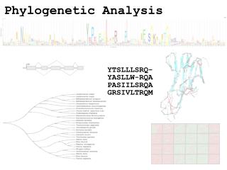
Phylogenetic Analysis 1
Phylogenetic Analysis 1. Phylogeny (phylo =tribe + genesis). What can be inferred from phylogenetic trees built from sequence data?. Which species are the closest living relatives of modern humans? Did the infamous Florida Dentist infect his patients with HIV?

Phylogenetic Analysis 1
E N D
Presentation Transcript
Phylogenetic Analysis 1 Phylogeny (phylo =tribe + genesis)
What can be inferred from phylogenetic trees built from sequence data? • Which species are the closest living relatives of modern humans? • Did the infamous Florida Dentist infect his patients with HIV? • What were the origins of specific transposable elements? • Plus countless others…..
Which species are the closest living relatives of modern humans? Mitochondrial DNA, most nuclear DNA-encoded genes, and DNA/DNA hybridization all show that bonobos and chimpanzees are related more closely to humans than either are to gorillas. Humans Gorillas Chimpanzees Chimpanzees Bonobos Bonobos Gorillas Orangutans Orangutans Humans 14 0 0 15-30 MYA MYA The pre-molecular view was that the great apes (chimpanzees, gorillas and orangutans) formed a clade separate from humans, and that humans diverged from the apes at least 15-30 MYA.
No No Did the Florida Dentist infect his patients with HIV? DENTIST Phylogenetic tree of HIV sequences from the DENTIST, his Patients, & Local HIV-infected People: Patient C Patient A Patient G Yes: The HIV sequences from these patients fall within the clade of HIV sequences found in the dentist. Patient B Patient E Patient A DENTIST Local control 2 Local control 3 Patient F Local control 9 Local control 35 Local control 3 Patient D From Ou et al. (1992) and Page & Holmes (1998)
What can be learned from character analysis using phylogenies? • When did specific episodes of positive Darwinian selection occur during evolutionary history? • Which genetic changes are unique to the human lineage? • What was the most likely geographical location of the common ancestor of the African apes and humans? • Plus countless others…..
What was the most likely geographical location of the common ancestor of the African apes and humans? Scenario A: Africa as species fountain Scenario B: Eurasia as ancestral homeland Scenario B requires four fewer dispersal events Eurasia = Black Africa = Red = Dispersal Modified from: Stewart, C.-B. & Disotell, T.R. (1998) Current Biology 8: R582-588.
How can we choose between competing hypotheses on phylogeny of whales?
Phylogenetic Reconstruction of Whales • Whales belong to artiodactyla (ungulate mammals), which includes camels, pigs, hippos, cows, deer • Outgroup is rhinos/horses • Difficult to place them because they lack many characters present in terrestrial mammals (e.g. hind limbs) • Are whales sister to entire group or to hippos?
DNA Sequence Data and Whale Evolution • Data collected from beta-casein gene for all taxa and sequences aligned. • Nucleotide changes between outgroup and ingroup species indicate shared derived homologies. • Most nucleotides are identical in all taxa, these are uninformative for phylogeny. • Some nucleotides indicate that whales belong with cows, deer, and hippos (162). • Others indicate that whales and hippos are sister groups (166). • Others contradict sister group status of whale/hippo and cow deer (177) and may indicate a reversal.
Problems in Reconstructing Phylogeny • Characters sometimes conflict • It is sometimes difficult to tell homology from homoplasy • Analogy- characters similar because of convergent evolution • Reversal- character reverts to ancestral form • With morphological characters, careful examination may distinguish homoplasy (orthologs) from homology • With molecular characters (DNA/Protein sequences), orthologs sometimes impossible to distinguish from homologs and paralogs.
A Phylogenetic Tree • Taxon -- Any named group of organisms – evolutionary theory not necessarily involved. • Clade -- A monophyletic taxon (evolutionary theory utilized)
A phylogenetic tree with branch lengths • Branch length can be significant… • In this case it is and mouse is slightly more similar to fly than human is to fly (sum of branches 1+2+3 is less than sum of 1+2+4)
Common Phylogenetic Tree Terminology Terminal Nodes Branches or Lineages A Represent the TAXA (genes, populations, species, etc.) used to infer the phylogeny B C D Ancestral Node or ROOT of the Tree E Internal Nodes or Divergence Points (represent hypothetical ancestors of the taxa)
Taxon B Taxon C No meaning to the spacing between the taxa, or to the order in which they appear from top to bottom. Taxon A Taxon D Taxon E This dimension either can have no scale (for ‘cladograms’), can be proportional to genetic distance or amount of change (for ‘phylograms’ or ‘additive trees’), or can be proportional to time (for ‘ultrametric trees’ or true evolutionary trees). Phylogenetic trees diagram the evolutionary relationships between the taxa ((A,(B,C)),(D,E)) = The above phylogeny as nested parentheses These say that B and C are more closely related to each other than either is to A, and that A, B, and C form a clade that is a sister group to the clade composed of D and E. If the tree has a time scale, then D and E are the most closely related.
time Three types of trees Cladogram Phylogram Ultrametric tree 6 Taxon B Taxon B Taxon B 1 1 Taxon C Taxon C Taxon C 3 1 Taxon A Taxon A Taxon A Taxon D Taxon D 5 Taxon D no meaning genetic change All show the same evolutionary relationships, or branching orders, between the taxa.
cladogram t1 • relative recenct common descent. • Does not imply that ancestors on the same line necessarily speciated at the same time. • t1 can bebefore or after t2 but not before t3 t3 t2 Types of trees: cladogram (no time scale)
branch lengths = amount of change Types of trees: phylogram phylogram (additive tree: branch lenghts can be summed) relative recenct common descent, and
divergence Types of trees: ultrametric Ultrametric tree (linearized tree) All tree tips are equidistant from the root Amount of change can be scaled to time scale = time
A A A B C E C E C D B B E D D Polytomy or multifurcation A bifurcation The goal of phylogeny inference is to resolve the branching orders of lineages in evolutionary trees Completely unresolved or "star" phylogeny Partially resolved phylogeny Fully resolved, bifurcating phylogeny
There are three possible unrooted trees for four taxa (A, B, C, D) Tree 1 Tree 2 Tree 3 A C A B A B D D C D B C Phylogenetic tree building (or inference) methods are aimed at discovering which of the possible unrooted trees is "correct". We would like this to be the “true” biological tree — that is, one that accurately represents the evolutionary history of the taxa. However, we must settle for discovering the computationally correct or optimal tree for the phylogenetic method of choice.
A B A C C D B C D A E B C A D E B F The number of unrooted trees increases in a greater than exponential manner with number of taxa (2N - 5)!! = # unrooted trees for N taxa
B C Root D A A C B D Rooted tree Note that in this rooted tree, taxon A is no more closely related to taxon B than it is to C or D. Root Inferring evolutionary relationships between the taxa requires rooting the tree: To root a tree mentally, imagine that the tree is made of string. Grab the string at the root and tug on it until the ends of the string (the taxa) fall opposite the root: Unrooted tree
Try it again with the root at another position B C Root Unrooted tree D A A B B C D Rooted tree Note that in this rooted tree, taxon A is most closely related to taxon B, and together they are equally distantly related to taxa C and D. Root
2 4 1 5 3 Rooted tree 1a Rooted tree 1b Rooted tree 1c Rooted tree 1d Rooted tree 1e B A A C D A B D C B C C C A A D B B D D An unrooted, four-taxon tree theoretically can be rooted in five different places to produce five different rooted trees A C The unrooted tree 1: D B These trees show five different evolutionary relationships among the taxa!
Sometimes two trees may look very different but, in fact, differ only in the position of the root
A A C D D B C B B A B C C D D A C B D D A C B A All of these rearrangements show the same evolutionary relationships between the taxa Rooted tree 1a D C A B
There are two major ways to root trees By outgroup: Uses taxa (the “outgroup”) that are known to fall outside of the group of interest (the “ingroup”). Requires some prior knowledge about the relationships among the taxa. The outgroup can either be species (e.g., birds to root a mammalian tree) or previous gene duplicates (e.g., a-globins to root b-globins). outgroup By midpoint or distance: Roots the tree at the midway point between the two most distant taxa in the tree, as determined by branch lengths. Assumes that the taxa are evolving in a clock-like manner. This assumption is built into some of the distance-based tree building methods. A d (A,D) = 10 + 3 + 5 = 18 Midpoint = 18 / 2 = 9 10 C 3 2 2 B D 5
Rooting Using an Outgroup • The outgroup should be a sequence (or set of sequences) known to be less closely related to the rest of the sequences than they are to each other. • It should ideally be as closely related as possible to the rest of the sequences while still satisfying the first condition. • The root must be somewhere between the outgroup and the rest (either on the node or in a branch).
Automatic rooting • Many software packages will root trees automatically (e.g. mid-point rooting in NJPlot) • This normally involves assumptions… BEWARE!
C A x = D B C A D B E C A D E B F (2N - 3)!! = # unrooted trees for N taxa Each unrooted tree theoretically can be rooted anywhere along any of its branches
COMPUTATIONAL METHOD Optimality criterion Clustering algorithm PARSIMONY MAXIMUM LIKELIHOOD Characters DATA TYPE MINIMUM EVOLUTION LEAST SQUARES UPGMA NEIGHBOR-JOINING Distances Molecular phylogenetic tree building methods Are mathematical and/or statistical methods for inferring the divergence order of taxa, as well as the lengths of the branches that connect them. There are many phylogenetic methods available today, each having strengths and weaknesses. Most can be classified as follows:
Types of data used in phylogenetic inference Character-based methods:Use the aligned characters, such as DNA or protein sequences, directly during tree inference. TaxaCharacters Species A ATGGCTATTCTTATAGTACG Species B ATCGCTAGTCTTATATTACA Species C TTCACTAGACCTGTGGTCCA Species D TTGACCAGACCTGTGGTCCG Species E TTGACCAGTTCTCTAGTTCG Distance-based methods:Transform the sequence data into pairwise distances (dissimilarities), and then use the matrix during tree building. A B C D E Species A ---- 0.20 0.50 0.45 0.40 Species B 0.23 ---- 0.40 0.55 0.50 Species C 0.87 0.59 ---- 0.15 0.40 Species D 0.73 1.12 0.17 ---- 0.25 Species E 0.59 0.89 0.61 0.31 ---- Example 1: Uncorrected “p” distance (=observed percent sequence difference) Example 2: Kimura 2-parameter distance (estimate of the true number of substitutions between taxa)
6 Taxon B 1 1 Taxon C 3 1 Taxon A 5 Taxon D C is more similar in sequence to A (d = 3) than to B (d = 7), but C and B are most closely related (that is, C and B shared a common ancestor more recently than either did with A). Similarity vs. Evolutionary Relationship Similarity and relationship are not the same thing, even though evolutionary relationship is inferred from certain types of similarity. Similar: having likeness or resemblance (an observation) Related: genetically connected (an historical fact) Two taxa can be most similar without being most closely-related:
C C G G C G G C Types of Similarity Observed similarity between two entities can be due to: Evolutionary relationship: Shared ancestral characters (‘plesiomorphies’) Shared derived characters (‘’synapomorphy’) Homoplasy (independent evolution of the same character): Convergent events (in either related on unrelated entities), Parallel events (in related entities), Reversals (in related entities) G C C G T G C G Character-based methods can tease apart types of similarity and theoretically find the true evolutionary tree. Similarity = relationship only if certain conditions are met (if the distances are ‘ultrametric’).
a 9 6 5 b c METRIC DISTANCES between any two or three taxa (a, b, and c) have the following properties: Property 1: d (a, b) ≥ 0 Non-negativity Property 2: d (a, b) = d (b, a) Symmetry Property 3: d (a, b) = 0 if and only if a = b Distinctness Property 4: d (a, c) ≤ d (a, b) + d (b, c) Triangle inequality:
4 a b 6 6 c a 2 2 2 b 4 c ULTRAMETRIC DISTANCES must satisfy the previous four conditions, plus: Property 5 d (a, b) ≤ maximum [d (a, c), d (b, c)] This implies that the two largest distances are equal, so that they define an isosceles triangle: Similarity = Relationship if the distances are ultrametric! If distances are ultrametric, then the sequences are evolving in a perfectly clock-like manner, thus can be used in UPGMA trees and for the most precise calculations of divergence dates.
ADDITIVE DISTANCES: Property 6: d (a, b) + d (c, d) ≤ maximum [d (a, c) + d (b, d), d (a, d) + d (b, c)] For distances to fit into an evolutionary tree, they must be either metric or ultrametric, and they must be additive. Estimated distances often fall short of these criteria, and thus can fail to produce correct evolutionary trees.
Clustering algorithms: • Use pairwise distances. • Are purely algorithmic methods, in which the algorithm itself defines the the tree selection criterion. • Tend to be very fast programs that produce singular trees rooted by distance. • No objective function to compare to other trees, even if numerous other trees could explain the data equally well. • Warning: Finding a singular tree is not necessarily the same as finding the "true” evolutionary tree.
Optimality approaches: • Use either character or distance data. • First define an optimality criterion (minimum branch lengths, fewest number of events, highest likelihood), and then use a specific algorithm for finding trees with the best value for the objective function. • Can identify many equally optimal trees, if such exist. • Warning: Finding an optimal tree is not necessarily the same as finding the "true” tree.
Computational methods for finding optimal trees: Exact algorithms:"Guarantee" to find the optimal or "best" tree for the method of choice. Two types used in tree building: Exhaustive search: Evaluates all possible unrooted trees, choosing the one with the best score for the method. Branch-and-bound search: Eliminates the parts of the search tree that only contain suboptimal solutions. Heuristic algorithms: Approximate or “quick-and-dirty” methods that attempt to find the optimal tree for the method of choice, but cannot guarantee to do so. Heuristic searches often operate by “hill-climbing” methods.
A B A C C D B C D A E B C A D E B F Exact searches become increasingly difficult, and eventually impossible, as the number of taxa increases: (2N - 5)!! = # unrooted trees for N taxa
Heuristic search algorithms are input order dependent and can get stuck in local minima or maxima Rerunning heuristic searches using different input orders of taxa can help find global minima or maxima Search for global maximum Search for global minimum GLOBAL MAXIMUM GLOBAL MAXIMUM local maximum local minimum GLOBAL MINIMUM GLOBAL MINIMUM
Assumptions made by phylogenetic methods: • The sequences are correct • The sequence are homologous • Each position is homologous • The sampling of taxa or genes is sufficient to resolve the problem of interest • Sequence variation is representative of the broader group of interest • Sequence variation contains sufficient phylogenetic signal (as opposed to noise) to resolve the problem of interest • Each position in the sequence evolved independently
Problems with Phylogenetic Inference • How do we know what the potential candidate trees are? • How do we choose which tree is (most likely) the true tree?
Recipe for reconstructing a phylogeny • Select an optimality criterion • Select a search strategy • Use the selected search strategy to generate a series of trees, and apply the selected optimality criterion to each tree, always keeping track of the “best” tree examined thus far. • How do you know the “best” tree? • Which is the “true” tree?
Search strategy: Which is the right tree? • When m is the number of taxa, the number of possible trees is: • [(2m-3)!]/[2m-2(m-2)!] • For 10 taxa, the number of trees is 34,459,425 • Many trees can be discarded because they are obviously wrong • Sometimes, there is a general or even specific grouping that can serve as a start for the tree search • There are a number of approaches to tree searches that can be used