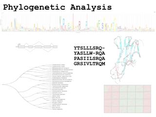
Phylogenetic Analysis

1. Phylogenetic Analysis

2. Introduction • Intension • Using powerful algorithms to reconstruct the evolutionary history of all know organisms. • Phylogenetic tree • It can help understand the evolutionary relationships among species of organisms. • But we have to infer the evolutionary history of current organisms.

3. Campanulaceae (bluebell) family Herpesviruses

4. Common Phylogenetic Tree Terminology Terminal Nodes Branches or Lineages A Represent the TAXA (genes, populations, species, etc.) used to infer the phylogeny B C D Ancestral Node or ROOT of the Tree E Internal Nodes or Divergence Points (represent hypothetical ancestors of the taxa)

5. time Three types of trees Cladogram Phylogram Ultrametric tree 6 Taxon B Taxon B Taxon B 1 1 Taxon C Taxon C Taxon C 3 1 Taxon A Taxon A Taxon A Taxon D Taxon D 5 Taxon D no meaning genetic change All show the same evolutionary relationships, or branching orders, between the taxa.

6. Taxon B Taxon C No meaning to the spacing between the taxa, or to the order in which they appear from top to bottom. Taxon A Taxon D Taxon E This dimension either can have no scale (for ‘cladograms’), can be proportional to genetic distance or amount of change (for ‘phylograms’ or ‘additive trees’), or can be proportional to time (for ‘ultrametric trees’ or true evolutionary trees). Phylogenetic trees diagram the evolutionary relationships between the taxa ((A,(B,C)),(D,E)) = The above phylogeny as nested parentheses These say that B and C are more closely related to each other than either is to A, and that A, B, and C form a clade that is a sister group to the clade composed of D and E. If the tree has a time scale, then D and E are the most closely related.

7. A A A B C E C E C D B B E D D Polytomy or multifurcation A bifurcation The goal of phylogeny inference is to resolve the branching orders of lineages in evolutionary trees: Completely unresolved or "star" phylogeny Partially resolved phylogeny Fully resolved, bifurcating phylogeny

8. There are three possible unrooted trees for four taxa (A, B, C, D) Tree 1 Tree 2 Tree 3 A C A B A B D D C D B C Phylogenetic tree building (or inference) methods are aimed at discovering which of the possible unrooted trees is "correct". We would like this to be the “true” biological tree — that is, one that accurately represents the evolutionary history of the taxa. However, we must settle for discovering the computationally correct or optimal tree for the phylogenetic method of choice. C-B Stewart, NHGRI lecture, 12/5/00

9. A B A C C D B C D A E B C A D E B F The number of unrooted trees increases in a greater than exponential manner with number of taxa (2N - 5)!! = # unrooted trees for N taxa (2N- 3)!! = # rooted trees for N taxa

10. y x y y y x x x z z z z Introduction • NP-Hard optimization problem • Unrooted trees # of n organisms = TU(n) • Edges # of unrooted trees of n organisms = E(n)= 2n-3 , n>=2 • TU(n) = TU(n-1)*E(n-1) = ΠE(i) = Π(2i-5) • Ex. • Rooted trees # of n organisms = TR(n)= TU(n)*E(n) = TU(n+1) n-1 n i=2 i=3 add t t t t

11. B C Root D A A C B D Rooted tree Note that in this rooted tree, taxon A is no more closely related to taxon B than it is to C or D. Root Inferring evolutionary relationships between the taxa requires rooting the tree: To root a tree mentally, imagine that the tree is made of string. Grab the string at the root and tug on it until the ends of the string (the taxa) fall opposite the root: Unrooted tree

12. Now, try it again with the root at another position: B C Root Unrooted tree D A A B C D Rooted tree Note that in this rooted tree, taxon A is most closely related to taxon B, and together they are equally distantly related to taxa C and D. Root

13. 2 4 1 5 3 Rooted tree 1a Rooted tree 1b Rooted tree 1c Rooted tree 1d Rooted tree 1e B A A C D A B D C B C C C A A D B B D D An unrooted, four-taxon tree theoretically can be rooted in five different places to produce five different rooted trees A C The unrooted tree 1: D B These trees showfive different evolutionary relationships among the taxa!

14. A A C D D B C B B A B C C D D A C B D D A C B A All of these rearrangements show the same evolutionary relationships between the taxa Rooted tree 1a D C A B

15. COMPUTATIONAL METHOD Optimality criterion Clustering algorithm PARSIMONY MAXIMUM LIKELIHOOD Characters DATA TYPE MINIMUM EVOLUTION LEAST SQUARES UPGMA NEIGHBOR-JOINING Distances Molecular phylogenetic tree building methods: Are mathematical and/or statistical methods for inferring the divergence order of taxa, as well as the lengths of the branches that connect them. There are many phylogenetic methods available today, each having strengths and weaknesses. Most can be classified as follows:

16. parsimony • model complexity vs. sample size • minimize Hamming distance summed over all edges of the tree • justification: minimum possible number of evolutionary events • subject of serious dispute by systematic biologists

17. AAA AAA AAA AAA AAA AAA 1 1 2 1 2 1 GGA AGA GGA AGA AAG AAG AAA AAA Method • Maximum parsimony (MP) • Seek the tree that minimizes the total number of evolutionary events on the edges of tree • Ex. • Require two algorithms • Search over tree topology • The computation of a cost for a given tree AAA 1 AAA AGA 1 1 AAA AGA AAG GGA

18. maximum likelihood • estimate probability that a specific evolutionary model will produce a particular phylogeny yielding the observed sequences • many evolutionary models

19. Method • Maximum likelihood (ML) • Seek the tree that maximizes likelihood P(data|tree) • Ex. • Compute likelihoodP(x1,x2,x3|T,t1,t2,t3,t4) • x•: a set of sequences • T: a tree • t•: edge lengths of tree • Require two algorithms • Search over tree topology • Search over all possible lengths of edges t• to compute likelihood root X5 t4 X4 t3 t2 t1 X2 X1 X3

20. Distance Matrix Methods • produce a tree such that the path distance between leaves i and j (sum of edge weights in the path between i and j) equals Dij • this the additive property for a distance matrix -- of course real distance matrices may not be additive • most methods use agglomerative clustering -- successively choosing pairs of nodes to combine

21. Ultrametric trees • path distance from the root to each leaf is the same • strong molecular clock assumption - distance is proportional to evolutionary time

22. Example Tree and Additive Matrix

23. Distance Matrix Methods • UPGMA • Neighbor Joining • Fitch Margoliash • Quartet Puzzling • Witness-Anitwitness • Double Pivotmany are “not yet in use by the systematic biology community”

24. Distance Measures • DNA hybridization amounts • immunological distances • genetic distances • sequence distances (DNA, RNA, protein)

25. …what distance? • need distance measure that reflects the actual number of point mutations on the path between the leaves • particular problem with sequence data - Hamming distance and assumption of no reversals

26. UPGMA • Unweighted Pair-Group Method with Arithmetic mean

27. UPGMA Step 1combine B and C

28. UPGMA step 2combine BC and D (10+12)/2 (4+6)/2

29. 2 .5 0.5 d a 2 2 e b c UPGMA step 3combine A and E

30. UPGMA step 4combine AE and BCD

31. UPGMA Result 3.5

32. UPGMA Result 3.5

33. Method • Phylogenetic reconstruction techniques • NJ (neighbor-joining method) • A star tree is successively inserted branches between a pair of closest neighbors and the remaining terminals in the tree • Character • The fastest reconstruction method • Poor accuracy when the distance matrix contains large value

34. S1 S3 3.67 4 5 3.33 X S2 S4 S1 X S2 S1 S3 X S2 S4 Method • Ex. • The cost save by pairing S1 and S2 = New connection cost (NC) – Old connection cost (OC) = 2.34 NC = ½(average(S1)+average(S2)+d(S1,S2))=6.33 OC = average(S1) +average(S2) = 8.67 • The largest cost save by pairing S3 and S4 = 2.67Thus we pair S3 and S4 Distance matrix Star tree Pair S1 and S2

35. Neighbor-Joining Result

36. Genome Rearragement • Generalized Nadean-Tayor (GNT) evolution model • P(transpostion) = α • P(inverted trans.) = β • P(inversion) = 1-(α+β) • events # on edge :according to Poissondistributionf(x) = ; x=1,2,.. λx•e-3 x! Genome rearrangement

37. Improving reconstruction algorithms

38. Improving reconstruction algorithms • Estimators of true evolutionary distance • Exact-IEBP (inverting the expected breakpoint distance)ML estimate of the breakpoint distance after K rearrangements • Approx-IEBPapproximate Exact-IEBP • EDE (empirically derived estimator)empirical estimate of the inversion distance after K rearrangements produced a nonlinear regression formula that computes the expected distance given that K random rearrangements

39. Conclusion • New generation of phylogenetic software needs • More sophisticated models of evolution • Faster optimization algorithms • High performance algorithm engineering • Powerful modes of user interaction