Download
1 / 105
1.05k likes | 1.18k Vues
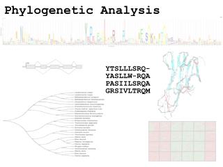
Explore DNA-RNA transcription, protein sequence data handling, and numerical comparisons using Perl scripts. Enhance knowledge of phylogenetic analysis for evolutionary tree reconstruction.

E N D
#!/usr/bin/perl -w $DNA1 = 'ACGGGAGGACGGGAAAATTACTACGGCATTAGC'; $DNA2 = 'ATAGTGCCGTGAGAGTGATGTAGTA'; $DNA3 = "$DNA1$DNA2"; $DNA4 = $DNA1 . $DNA2; exit;
#!/usr/bin/perl –w $DNA = 'ACGGGAGGACGGGAAAATTACTACGGCATTAGC'; print "Here is the starting DNA:\n\n"; print "$DNA\n\n"; # Transcribe the DNA to RNA by substituting all T's with U's. $RNA = $DNA; $RNA =~ s/T/U/g; # Print the RNA onto the screen print "Here is the result of transcribing the DNA to RNA:\n\n"; print "$RNA\n"; # Exit the program. exit;
#!/usr/bin/perl -w # The filename of the file containing the protein sequence data $proteinfilename = 'NM_021964fragment.pep'; # First we have to "open" the file open(PROTEINFILE, $proteinfilename); $protein = <PROTEINFILE>; # Now that we've got our data, we can close the file. close PROTEINFILE; # Print the protein onto the screen print "Here is the protein:\n\n"; print $protein; exit;
#!/usr/bin/perl -w # The filename of the file containing the protein sequence data $proteinfilename = 'NM_021964fragment.pep'; # First we have to "open" the file open(PROTEINFILE, $proteinfilename); # Read the protein sequence data from the file, and store it # into the array variable @protein @protein = <PROTEINFILE>; # Print the protein onto the screen print @protein; # Close the file. close PROTEINFILE; exit;
#!/usr/bin/perl -w # array indexing @bases = ('A', 'C', 'G', 'T'); print "@bases\n"; print $bases[0], "\n"; print $bases[1], "\n"; print $bases[2], "\n"; print $bases[3], "\n"; exit;
#!/usr/bin/perl -w $proteinfilename = 'NM_021964fragment.pep'; open(PROTEINFILE, $proteinfilename); $protein = <PROTEINFILE>; close PROTEINFILE; chomp $protein; $len = length $protein; print $len, ""; exit;
#!/usr/bin/perl -w $name = "PALLAPP"; $st1 = substr($name, 3); $st2 = substr($name, 1, 2);
Comparison • String comparison (are they the same, > or <) • eq (equal ) • ne(not equal ) • ge(greater or equal ) • gt (greater than ) • lt(less than ) • le(less or equal )
But • Use ==, <, <=, >, >=, !=, ||, && for numeric numbers • Use eq, lt, le, gt, ge, ne, or, and for string comparisons
$x = 10; $y = -20; if ($x le 10) { print "1st true\n";} if ($x gt 5) {print "2nd true\n";} if ($x le 10 || $y gt -21) {print "3rd true\n";} if ($x gt 5 && $y lt 0) {print "4th true\n";} if (($x gt 5 && $y lt 0) || $y gt 5) {print "5th true\n";}
#!/usr/bin/perl -w $num = 1234; $str = '1234'; print $num, " ", $str, "\n"; $num_or_str = $num + $str; print $num_or_str, "\n"; $num_or_str = $num . $str; print $num_or_str, "\n"; exit;
More Arithmatics • +, -, *, **, /, % • +=, -=, *=, **=, /=, %= • ++, --
$x = 10; $x = $x*1.5; print $x*=3, "\n"; print $x++, "\n"; print $x, "\n"; print ++$x, "\n"; print $x, "\n"; print $x % 3, "\n"; print $x**2, "\n";
$DNA = "ACCTAAACCCGGGAGAATTCCCACCAATTCTACGTAAC"; $s = ""; for ($i = 0, $j = 5; $i < $j; $i+=2, $j++) { $s .= substr($DNA, $i, $j); } print $s, "\n";
sub extract_sequence_from_fasta_data { my(@fasta_file_data) = @_; my $sequence = ''; foreach my $line (@fasta_file_data) { if ($line =~ /^\s*$/) { next; } elsif($line =~ /^\s*#/) { next; } elsif($line =~ /^>/) { next; } else { $sequence .= $line; } } # remove non-sequence data (in this case, whitespace) from $sequence string $sequence =~ s/\s//g; return $sequence; }
Human Migration Out of Africa 1. Yorubans 2. Western Pygmies 3. Eastern Pygmies 4. Hadza 5. !Kung 1 2 3 4 5 http://www.becominghuman.org
New Map 1 2 3 4 5
Additive Distance Matrices Matrix D is ADDITIVE if there exists a tree T with dij(T) = Dij NON-ADDITIVE otherwise
The Four Point Condition (cont’d) Compute: 1. Dij + Dkl, 2. Dik + Djl, 3. Dil + Djk 2 3 1 2 and 3 represent the same number: the length of all edges + the middle edge (it is counted twice) 1 represents a smaller number: the length of all edges – the middle edge
The Four Point Condition: Theorem • The four point condition for the quartet i,j,k,l is satisfied if two of these sums are the same, with the third sum smaller than these first two • Theorem : An n x n matrix D is additive if and only if the four point condition holds for every quartet 1 ≤ i,j,k,l ≤ n
Distance Based Phylogeny Problem • Goal: Reconstruct an evolutionary tree from a distance matrix • Input: n x n distance matrix Dij • Output: weighted tree T with n leaves fitting D • If D is additive, this problem has a solution and there is a simple algorithm to solve it
Find neighboring leavesi and j with parent k Remove the rows and columns of i and j Add a new row and column corresponding to k, where the distance from k to any other leaf m can be computed as: Using Neighboring Leaves to Construct the Tree Dkm = (Dim + Djm – Dij)/2 Compress i and j into k, iterate algorithm for rest of tree
D Q
D Q
D Q
Programs • BIONJ • WEIGHBOR • FastME
UPGMA: Unweighted Pair Group Method with Arithmetic Mean • UPGMA is a clustering algorithm that: • computes the distance between clusters using average pairwise distance • assigns a height to every vertex in the tree, effectively assuming the presence of a molecular clock and dating every vertex
Correct tree UPGMA 3 2 4 1 3 4 2 1 UPGMA’s Weakness: Example
Character-Based Tree Reconstruction • Better technique: • Character-based reconstruction algorithms use the n x m alignment matrix (n = # species, m = #characters) directly instead of using distance matrix. • GOAL: determine what character strings at internal nodes would best explain the character strings for the n observed species
Character-Based Tree Reconstruction (cont’d) • Characters may be nucleotides, where A, G, C, T are states of this character. Other characters may be the # of eyes or legs or the shape of a beak or a fin. • By setting the length of an edge in the tree to the Hamming distance, we may define the parsimony score of the tree as the sum of the lengths (weights) of the edges
Parsimony Approach to Evolutionary Tree Reconstruction • Applies Occam’s razor principle to identify the simplest explanation for the data • Assumes observed character differences resulted from the fewest possible mutations • Seeks the tree that yields lowest possible parsimony score - sum of cost of all mutations found in the tree
Small Parsimony Problem • Input: Tree T with each leaf labeled by an m-character string. • Output: Labeling of internal vertices of the tree T minimizing the parsimony score. • We can assume that every leaf is labeled by a single character, because the characters in the string are independent.
Weighted Small Parsimony Problem • A more general version of Small Parsimony Problem • Input includes a k * k scoring matrix describing the cost of transformation of each of k states into another one • For Small Parsimony problem, the scoring matrix is based on Hamming distance dH(v, w) = 0 if v=w dH(v, w) = 1 otherwise
Scoring Matrices Small Parsimony Problem Weighted Parsimony Problem
Unweighted vs. Weighted Small Parsimony Scoring Matrix: Small Parsimony Score: 5
Unweighted vs. Weighted Weighted Parsimony Scoring Matrix: Weighted Parsimony Score: 22
Weighted Small Parsimony Problem: Formulation • Input: Tree T with each leaf labeled by elements of a k-letter alphabet and a k x k scoring matrix (ij) • Output: Labeling of internal vertices of the tree T minimizing the weighted parsimony score
Check children’s every vertex and determine the minimum between them An example Sankoff’s Algorithm
Sankoff Algorithm: Dynamic Programming • Calculate and keep track of a score for every possible label at each vertex • st(v) = minimum parsimony score of the subtree rooted at vertex v if v has character t • The score at each vertex is based on scores of its children: • st(parent) = mini {si( left child) + i, t} + minj {sj( right child) + j, t}
Sankoff Algorithm (cont.) • Begin at leaves: • If leaf has the character in question, score is 0 • Else, score is
Sankoff Algorithm (cont.) st(v) = mini {si(u) + i, t} + minj{sj(w) + j, t} sA(v) = mini{si(u) + i, A} + minj{sj(w) + j, A} sA(v) = 0
Sankoff Algorithm (cont.) st(v) = mini {si(u) + i, t} + minj{sj(w) + j, t} sA(v) = mini{si(u) + i, A} + minj{sj(w) + j, A} sA(v) = 0 + 9 = 9
Sankoff Algorithm (cont.) st(v) = mini {si(u) + i, t} + minj{sj(w) + j, t} Repeat for T, G, and C
Sankoff Algorithm (cont.) Repeat for right subtree
Sankoff Algorithm (cont.) Repeat for root