Long Short Portfolio Optimisation under Mean-Variance-CVaR Framework
550 likes | 921 Vues
Long Short Portfolio Optimisation under Mean-Variance-CVaR Framework . Gautam Mitra CARISMA, Brunel University and OptiRisk systems, UK Diana Roman CARISMA, Brunel University and OptiRisk systems, UK Ritesh Kumar Indian Institute of Management, Calcutta, India. Outline.

Long Short Portfolio Optimisation under Mean-Variance-CVaR Framework
E N D
Presentation Transcript
Long Short Portfolio Optimisation underMean-Variance-CVaR Framework Gautam Mitra CARISMA, Brunel University and OptiRisk systems, UK Diana Roman CARISMA, Brunel University and OptiRisk systems, UK Ritesh Kumar Indian Institute of Management, Calcutta, India
Portfolio selection problem Initial Amount of capital to invest, n asset in which investment can be made. xj : The proportion of wealth invested in asset j Portfolio x=(x1,…,xn) has return Rx=x1R1+…+xnRn (Rx random variable). Another portfolio y=(y1,…,yn), has return Ry=y1R1+…+ynRn (Ry random variable) How do we choose between Rx and Ry? Problem of deciding between Random variables when larger outcomes are preferred. Preliminaries
Portfolio selection problem Discrete case: Use of Scenario models to obtain a representation for Random variables Rx when making portfolio choice x. Consider the case of T scenarios. pi=probability of scenario i occurring; p1+p2+…+pT=1 rij = return of asset j in scenario i; So asset j return Rj finitely distributed over {r1j, r2j,…,rTj} The portfolio return Rx finitely distributed over {R1x,…,RTx} Where Rix = x1ri1+…+xnrin is the return in scenario i. Preliminaries
Mean Risk Models Defining a preference relation for choosing a Random Variable Distributions are described and compared using Mean and value of a risk measure In the mean-risk approach,RX is preferred to r.v. RY (or RXdominates RY) if and only if it has greater expected value and less risk Let be a risk measure: a function mapping random variables into real numbers. RX is preferred to r.v. RY : (E(RX)E(RY) and (RX)(RY)) with at least one strict inequality. Preliminaries
Mean Risk Models The efficient (non-dominated) solutions are the Pareto optimal solutions of a two objective problem: Max (E(RX), -(RX)) Subject to: xP P=the set of feasible decision vectors Optimisation approach (One possible approach, not the only one!! ) Min (RX) Subject to: E(RX)d xP Preliminaries
Mean Risk Models • Pros: • Computationally convenient • Ready Interpretation of results • Cons: • Over simplified approach – Distribution described by just two • parameters! • Different risk measures – Different solutions • The question of what kind of risk measure to use is still open. Preliminaries
Risk Measures Dispersion Type of Risk Measures (Measure the deviation from a target) Symmetric risk measures: 1952: Variance (Markowitz): QP Model MAD: Due to computational difficulty of QP Models Not the case with the solvers today!! Asymmetric risk measures: Semi-Variance (Markowitz 1959) Lower partial moments (Bawa 1975, Fishburn 1977) Preliminaries
Risk Measures Several financial disasters raised the problem of hedging against worst case scenarios. • Risk measures concerned with the left tail of distributions: • VaR (1993, G-30& JP Morgan): although it has several important pitfalls, it is a standard in banking. • Difficult to optimise!!! • CVaR, also called “Expected Shortfall”, or “Tail VaR” (2000, Rockafellar and Uryasev): Attractive theoretical and computational properties. Preliminaries
Risk Measures Variance: Measures the spread around the expected value. Calculation: If Rx=x1R1+…+xnRn, then where ij= Cov(Ri,Rj) Thus, quadratic function of x1,…,xn Preliminaries
Risk Measures CVaR: Let A% =(0,1). CVaR at confidence level of Rx is the mathematical transcription of the concept “average of losses in the worst A% of cases”. Formally: CVaR is defined using -tail. The -tail distribution of Rx: the lower part of the distribution of Rx (corresponding to extreme unfavourable outcomes) with distribution function rescaled to span [0,1]. CVaR is minus the mean of the -tail distribution Preliminaries
Risk Measures CVaR Example: Rx a discrete random variable with 13 equally probable outcomes (arranged in ascending order) : -1, -0.75, -0.5, -0.25, -0.1, 0, 0.05, 0.1, 0.2, 0.3, 0.4, 0.5, 0.6 At =0.1 (1/13,2/13) consider the 2 worst outcomes. The -tail has outcomes –1 and –0.75 with probabilities 1/13:1/10=10/13 and 3/13. At =0.25 (3/13,4/13) consider the 4 worst outcomes. The -tail has outcomes –1, –0.75, -0.5 and –0.25 with probabilities 1/13:1/4=4/13, 4/13, 4/13 and 1/13. Preliminaries
Risk Measures CVaR Optimisation: CVaR is calculated and optimised using an auxiliary function (Rockafellar and Uryasev 2000). For discrete Random Variables, CVaR optimisation is a LP Where [u]+ =u for u0 and [u]+ =0 for u<0. Preliminaries
Risk Measures CVaR Calculation: CVaR Optimisation: Moreover: x* minimises CVaR over P v*R such that (x*,v*) minimises F(x,v) over PxR: Preliminaries
Motivation & Formulation • Variance still the most widely used risk measure by Fund Manager • CVaR is gaining popularity with Regulators • Risk quantification from different perspectives leads to different • solution portfolios when minimised. • Mean-Variance portfolio may have excessively large CVaR !! • Mean-CVaR portfolio may have excessively large variance !! • Our approach: Trade-off between Variance-CVaR. Distributions are • compared using 3 parameters: Mean, Variance and CVaR (Roman et al 2007). Mean-Variance-CVaR Model
Motivation&Formulation Preference relation: Rx is preferred to Ry (or the portfolio x is preferred to portfolio y) if: E(Rx)E(Ry), 2(Rx) 2(Ry), CVaR(Rx)CVaR(Ry) With at-least one strict inequality. The non-dominated (efficient) solutions are the Pareto optimal solutions of a three-objective problem: (MVC): max (E(Rx), -2(Rx), - CVaR(Rx)) Subject to: xP. Mean-Variance-CVaR Model
Optimisation approach • The -constraint methodin multi-objective optimisation: • Optimise one of the objective functions • Impose limits on the other ones and transform to constraints • We choose to optimiseVariance while limits are imposed on CVaR and Expected return. • Representing CVaR constraint: The same function F used for minimising CVaR may be used for imposing a constraint on CVaR, while • maximising the mean (Krokhmal et al., 2002) => F may be generally used for imposing a constraint on CVaR. Single objective problem Mean-Variance-CVaR Model
Optimisation approach (P): min 2(Rx) Subject to: F(x,v)z E(Rx)d xP, vR A QP Model !! If the covariance matrix is positive definite ( no replication of assets, no risk-free asset), and the constraints on mean and on CVaR are active, (P) is equivalent to (MVC). x*P is a Pareto efficient solution of (MVC) v*R such that (x*,v*) optimal solution of (P) with z= F(x*,v*), d= E(Rx*). Mean-Variance-CVaR Model
Model details i{1,…,T} i{1,…,T} (x1,…, xn)P Long Only Model
Obtaining Efficient Solution Sets • Varying the RHS in the constraints on mean and on CVaR such that these constraints are active produces the entire set of efficient solutions in the mean-variance-CVaR model. • d must be greater than the expected returns of both the minimum variance portfolio (mean-variance efficient) and the minimum CVaR portfolio (mean-CVaR efficient). • For d fixed, z must be less than the minimum CVaR of a mean-variance efficient portfolio with expected return d (for an active constraint); z must be greater than the minimum CVaR for expected return d (for feasibility). Long Only Model
Obtaining Efficient Solution Sets • Generally, the mean-variance and mean-CVaR efficient solutions are just particular solutions of (MVC). • But: if there are several mean-variance efficient portfolios with different CVaR-s, only the portfolio with the lowest CVaR is an efficient solution of (MVC). • If there are several mean-CVaR efficient portfolios with different variances, only the portfolio with the lowest variance is an efficient solution of (MVC). • Thus, (MVC) does not exclude mean-variance and mean-CVaR models but it “embeds” them. Long Only Model
Obtaining Efficient Solution Sets Long Only Model
Motivation- Short selling • In the Long only model - Portfolio weights are positive • Investors can sell short (portfolio weights can be negative) certain securities, which mean that they can sell investments that they do not currently own. • Long only portfolio focuses on “Winning securities” ignoring a whole class of “losing securities”. • A Long-Short portfolio expands the scope of the investor’s sphere of portfolio decisions -> Likely to improve performance than a Long only portfolio. • Active portfolio selection - Freedom from the restrictions imposed by individual securities’ benchmark weights. Short Selling in Practice
Short selling Constraints in Our Model • Net Margin Requirements as dictated by regulatory restrictions. • Regulation T specifies that the sum of long positions plus the sum of • short positions should not exceed twice the equity in the account. • Regulation T currently specifies H=2 Short Selling in Practice
Short selling Constraints in Our Model • Investor’s strategy: Investor may follow market neutral strategy or • full market exposure strategy with 120:20 strategy etc. • Total value of Long – Total value of short, be close to some investor • specified value, ν • Where τ represents a small non negative tolerance level. • For market neutral strategies ν = 0 • For full market exposure ν = 1 Short Selling in Practice
Short selling Constraints in Our Model • Budget Constraint • Short Rebate • When a security is sold short, the proceeds of the sale are deposited • with lender of the stock as collateral. The lender would invest that • money in some bank account which earns interest. After taking a • proportion of the interest, rest of the interest is passed back to the • investor (called short rebate). The percentage of interest that the • investor would get back depends on the negotiation. Short Selling in Practice
Short selling Constraints in Our Model • Long-Short positions can be modeled as mutual exclusive positions. • Threshold on individual long and short positions: Minimum level below • which an asset is not purchased or sold short. This requirement • eliminates the unrealistically small trades that can otherwise be • included in an optimized portfolio. Short Selling in Practice
Long-Short Model • We represent n assets using 2n non negative variables (n variables • representing long positions and n variables for short positions.) • Integrated Optimisation ofLong-Short positions (Jacobs et al 1999, 2006) • Variance for Long-Short positions • Co-variance Matrix for the integrated optimisation • Where Q represents the co-variance matrix between the n assets for long • only model Long-Short Model
Long-Short Model • Variance • Expected Return Long-Short Model
Long-Short Model • CVaR Long-Short Model
Cardinality constraint Cardinality constraint
Long-Short Model: Formulation for Scenario model Long-Short Model: Complete formulation
Long-Short Model: Formulation for Scenario model Long-Short Model: Complete formulation
Computational Results: Analysis and Discussion Dataset • 76 assets from FTSE 100 index • 132 time periods, considered as equally probable scenarios • Monthly returns: rij, i=1,…,T; j=1,…,n • Confidence level =0.01 • Short selling parameters • Return on cash( ) = 4% per annum • Short rebate ( ) = 80% • Full market exposure (ν=1) and 120:20 strategy, Tolerance τ=0 Computational Results: Analysis and Discussion
Computational Results: Analysis and Discussion • Portfolio selection models without cardinality constraint • Long-Short portfolio without cardinality: In Sample Analysis • Optimal Portfolios: Minimum and Maximum expected return • Considered expected return level = 0.0188 • At this expected return level we consider 5 portfolios efficient in MVC model including Mean-CVaR efficient portfolio and Mean-Variance efficient portfolios. Computational Results: Analysis and Discussion
Computational Results: Analysis and Discussion In-sample analysis, CVaR-variance plot, Expected return level of 0.0188 Computational Results: Analysis and Discussion
Computational Results: Analysis and Discussion Computational Results: Analysis and Discussion
Computational Results: Analysis and Discussion Computational Results: Analysis and Discussion
Computational Results: Analysis and Discussion • Long-short portfolio without cardinality: Out of Sample Analysis • Next 18 period Out of Sample data Computational Results: Analysis and Discussion
Computational Results: Analysis and Discussion Portfolio out-of-sample cumulative returns for 01-01-2004 to 06-01-2005 (In-sample portfolios constructed at expected return of 0.0188 and at different CVaR levels) Computational Results: Analysis and Discussion
Computational Results: Analysis and Discussion • Portfolio selection models with threshold and cardinality constraints • Lower limits on portfolio positions = 0.0001, Upper limit on portfolio positions = 1 • Long only model: In-sample analysis Computational Results: Analysis and Discussion
Computational Results: Analysis and Discussion Long only with threshold and cardinality constraints: Out-of-sample analysis Computational Results: Analysis and Discussion
Computational Results: Analysis and Discussion Long-short with threshold and cardinality constraints: In-sample analysis Computational Results: Analysis and Discussion
Computational Results: Analysis and Discussion Portfolios with threshold and cardinality constraints: In-sample plots Computational Results: Analysis and Discussion
Computational Results: Analysis and Discussion Long-short with threshold and cardinality constraints: Out-of-sample analysis Computational Results: Analysis and Discussion
Computational Results: Analysis and Discussion Portfolios with threshold and cardinality constraints: Out-of-sample cumulative returns Computational Results: Analysis and Discussion
Open issues – Our current research focus Mutual exclusivity of long and short positions – Is it really an industry requirement? Need further and deeper analysis of the properties of the efficient frontier. Margin requirements - A very simplistic treatment in this model. A better treatment under mean-variance framework given in Kwan (2004) We need to include the interest rates of borrowing and lending for the amount borrowed (For long positions) and amount deposited (For short sales). Investor’s strategy – What strategy do you follow? Is 120:20 strategy used in practice? Open issues
Conclusions • In MVC model we try to address both classical fund manager’s and regulator’s point of view. • Distributions compared using 3 statistics: Mean, Variance and CVaR. • The Mean-Variance and Mean-CVaR models are “embedded” but the MVC model discriminates “positively” between Mean-Variance solutions with different CVaR levels. • Some solutions (excluded by classical mean-risk models) may be an improvement: better left tail than mean-variance efficient distributions + smaller variance than mean-CVaR efficient distributions. • Long-Short optimisation able to achieve superior optimal portfolios at same return level: lower CVaR and Variance. Conclusions
References Jacobs, B., I Levy K.N. , Starer, D. (1999). "Long-Short Portfolio Management: An Integrated Approach." The Journal of Portfolio Management. Jacobs, B., I Levy K.N., Markowitz,H.M. (2006). "Trimability and Fast Optimization of Long-Short Portfolios " Financial Analyst JournalVol:62(2). Krokhamal, P., Palmquist, J. and Uryasev, S. (2002): “Portfolio Optimisation with Conditional Value-at-Risk Objective and Constraints”.Journal of Risk, 4, 43-68 Kwan, Clarence C.Y. (2004): “Long-short portfolio modeling: Critique and Extension”. International Journal of Theoretical and Applied Finance,Vol 7:1. Markowitz., H. M. (1952). "Portfolio selection." Journal of FinanceVol:7: 77-91. Rockafellar, R. T., Uryasev, S. (2000). "Optimization of Conditional Value at Risk." Journal of RiskVol:2: 21-42.
References… Roman, D., Mitra G., Darby-Dowman, K. (2007). "Mean-Risk Models Using Two Risk Measures: A Multi-Objective Approach.“ To appear in Quantitative Finance