Basic Block, Trace and Instruction Selection
Basic Block, Trace and Instruction Selection. Chapter 8 , 9. (1) Semantic gap. Tree IR. Machine Languages. (2) IR is not proper for optimization analysis. Tree representation => no execution order is assumed. Tree Model v.s. Flat list of instructions Eg:

Basic Block, Trace and Instruction Selection
E N D
Presentation Transcript
Basic Block, Traceand Instruction Selection Chapter 8, 9
(1) Semantic gap Tree IR Machine Languages (2) IR is not proper for optimization analysis • Tree representation => no execution order is assumed. • Tree Model v.s. Flat list of instructions • Eg: • - Some expressions have side effects • ESEQ ESEQ (rj M(rj+C), rk) , • CALL call(“f1”, ESEQ (rj M(rj+k), rk) , call(…)) • - Semantic Gap • CJUMP vs. Jump on Condition • 2 targets 1 target + “fall through” • (x>y) ? goto Ltrue : goto Lfalse vs. if(x>y) goto Ltrue
Semantic Gap Continued - ESEQ within expression is inconvenient - evaluation order matters - CALL node within expression causes side effect ! - CALL node within the argument – expression of other CALL nodes will cause problem if the args of result are passed in the same (one) register. - Rewrite Tree into an equivalent one(Canonical Form) SEQ S1 SEQ => S1;S2;S3;S4;S5 SEQ SEQ S2 S3 S4 S5
Transformation Step 1: A tree is rewritten into a list of “canonical trees” without SEQ or ESEQ nodes. -> tree.StmList linearize(tree.Stm S); Step 2: Grouping into a set of “basic blocks” which contains no internal jumps or labels -> BasicBlocks Step 3: Basic Blocks are ordered into a set of “traces” in which every CJUMP is immediately followed by false label. -> TraceSchedule(BasicBlocks b)
8.1 Canonical Trees • Def : canonical trees are those with following properties: • 1. No SEQ or ESEQ • remove ESEQ first and then SEQ • 2. The parent of each CALL is either • EXP(..) or MOVE(TEMP t, ….) • i.e., CALL(…) statement or • t CALL(…). • How to remove ESEQ? • Lifting ESEQ higher and higher until it becomes SEQ.
ESEQ ESEQ ESEQ e SEQ S1 e S2 S2 S1 Transformations on ESEQ -move ESEQ to higher level. Eg. Case 1: [S1 ; [S2 ; e ] ] [ [S1, S2]; e ]
Case 2: BINOP MEM JUMP CJUMP e2 op e l1 l2 op ESEQ ESEQ ESEQ ESEQ e1 e1 e1 e1 S S S S ESEQ ESEQ SEQ SEQ MEM BINOP S CJUMP JMP S S S e1 op e1 e2 op e1 e2 l1 l2 e1
MOVE e1 TEMP t Case 3: BINOP CJUMP op e1 ESEQ op e1 ESEQ ㅣ1 ㅣ2 e2 e2 S S1 ESEQ SEQ BINOP SEQ MOVE SEQ op TEMP e2 e1 S TEMP CJUMP S t t op TEMP e2 ㅣ1 ㅣ2 t
Case 4: When S does not affect e1 in case 3 and (s and e1 have no side effect( e.g., I/O)) CJUMP BINOP op e1 ESEQ ㅣ1 ㅣ2 op e1 ESEQ e2 S1 e2 S if s,e1 commute if s,e1 commute ESEQ SEQ S S BINOP CJUMP op e1 e2 op e1 e2 ㅣ1 ㅣ2
Some conditions under which twoExp/Stm commute: • 1. CONST(n) can commute with any Statement!! • 2. NOP (= ExpStm(CONST(0)) ) can commute with any Exp!! • Be Conservative if we cannot determine if two Exp/Stm • commute!! • Notation: [s1,…,sn : e1,…,em] ( n ≥ 0, m ≥ 0 ) • is a list of stms s1,…,sn followed by a list of Exps e1 … em. • Semantically it means we have to compute the list according to their order and return as a vector the • results of last m expressions.
General Rewriting Rules • Identify the subexpressions[e1,…,en] for each Exp • e or Stmt s. • ExpList kids() defined for each Exp and Stm. • e.g: Plus([s1 : e1],[s2 : e2 ]) --- e.kids() • [: [s1:e1],[s2:e2]] • Pull the ESEQs out of the stm or exp and rebuild. • e.g:[: [s1:e1],[s2,e2] ] --- reorder • [ s1,s2 : e1,e2] --- build([:e1,e2]) • [ s1,s2 : PLUS(e1,e2) ] --- new ESEQ(_,_). • ESEQ(SEQ(s1,s2), PLUS(e1,e2) ) • (Stm, ExpList ) reorder( ExpList ) ; • reorder([: e1,e2,…,em]) return[s1,s2,…,sn: e1,e2,…,em ] • Stm | Exp build(ExpList kids)
Additional example e =CALL( e1, e2, ESEQ(s1,e3) ) --- e.kids() [: e1,e2,ESEQ(s1,e3)] --- reorder(.) [ s1 : e1,e2,e3]if s1, e1,e2 commute or [ MOVE(t1,e1),s1 : TEMP(t1), e2, e3 ] elseif s1, e2 commute or [ MOVE(t1, e1),MOVE(t2,e2),s1 : TEMP(t1), TEMP(t2), e3 ]o/w --- build() [s1 : CALL(e1,e2,e3 ) ] or … --- new ESEQ() ESEQ(s1, CALL(e1,e2,e3)).
package canon; public class Canon { … static tree.Stm reorder_stm(tree.Stm s) { // StmExpList is a pair of Stm and ExpList. StmExpList x = reorder(s.kids()); // seq(a,b) return new SEQ(a,b). returnseq(x.stm, s.build(x.exps)); } static tree.ESEQ reorder_exp (tree.Exp e) { StmExpList x = reorder(e.kids()); returnnew tree.ESEQ(x.stm, e.build(x.exps)); }
Moving CALLS to Toplevel • All CALLs return their results in the same register (e.g, • TEMP( RV) in mips ). • CALL( obj,CALL(…),CALL(…)) results in conflict. Solution : 1. save every CALL result in a new temporary. CALL(fun,args) -> // t is a new temporary. ESEQ(MOVE(TEMP t,CALL(fun,args)),TEMP t) I.e., [: [ MOVE(TEMP t,CALL(fun,args)) : TEMP t ] ] • need extra TEMP(t) (registers) 2. Then eliminate/lifiting ESEQ. => [ MOVE(TEMP t,CALL(fun,args)) : TEMP t ] overwrite TEMP(RV)
do_stm(MOVE(TEMP tnew, CALL(f, args))) • do_stm (EXP(CALL(f, args))) • - will not reorder on CALL node • ( so infinite recursion can be avoided) • - will reorder on f and args as the children of MOVE
A LINEAR LIST OF STATEMENTS S0 S0’ (right linear) SEQ(a, SEQ(b, c)) => [a,b,c] SEQ SEQ a SEQ SEQ c a b b c linearlize(stm s0) :StmList
8.2 TAMING CONDITIONAL BRANCHES Definition : BASIC BLOCK : a sequence of statements entered at the beginning exited at the end - The 1st stmt is a LABEL - The last stmt is a JUMP or a CJUMP - no other LABELs, JUMPs, CJUMPs.. Cond CJUMP CJUMP T F Cond F: …… t T: . . . (C)JUMP LABEL
Partition a list of statements into basic blocks • Algorithm : Scan from beginning to end • - when Label is found, begin new Block (and end previous block) • - when JUMP or CJUMP is found, a block is ended ( an d begin the next block) • - If block begins w/o label add a label; • - If block ends without JUMP or CJUMP, insert two • statements : • JUMP LABEL • LABEL : • Epilogue block of Function. insert two stms at the end: • JUMP DONE: • DONE; • Note: The class canon.BasicBlocks implements this algorithm.
m 0 v 0 L3: if v >= n goto L15 r v s 0 if r < n goto L9 v v + 1 goto L3 L9: x M[r] s s + x if s <= m got L13 m s L13: r r + 1 goto L6 L15: rv m Example:
m 0 v 0 L3: if v >= n goto L15 r v s 0 if r < n goto L9 v v + 1 goto L3 L9: x M[r] s s + x if s <= m got L13 m s L13: r r + 1 goto L6 L15: rv m JUMP done Done: (function Epilogue) Example: (add epilogue and find end of blocks)
m 0 v 0 L3: if v >= n goto L15 r v s 0 if r < n goto L9 v v + 1 goto L3 L9: x M[r] s s + x if s <= m got L13 m s L13: r r + 1 goto L6 L15: rv m JUMP done Done: (function Epilogue) Example: (start of blocks)
Lb1: m 0 v 0 L3: if v >= n goto L15 Lb2: r v s 0 if r < n goto L9 Lb3: v v + 1 goto L3 L9: x M[r] s s + x if s <= m got L13 Lb4: m s L13: r r + 1 goto L6 L15: rv m JUMP done Done: (function Epilogue) Example: (insert start label)
Lb1: m 0 v 0 ; JUMP L3 L3: if v >= n goto L15 Lb2: r v s 0 if r < n goto L9 Lb3: v v + 1 goto L3 L9: x M[r] s s + x if s <= m got L13 Lb4: m s ; JUMP L13 L13: r r + 1 goto L6 L15: rv m JUMP done Done: (function Epilogue) Example: (insert ending JUMP)
Traces Definition : Trace: A trace isa sequence of statements(or blocks ) that could beconsecutively executed during the execution of the program. We want a set of traces that exactly covers the program : Every block belongs to exactly one one trace. To reduce JUMPs, fewer traces are preferred !! Exit
Idea : the greedy method 1 1 T 2 2 F T F 3 3 4 4 F T T F 5 5 6 6 JUMP 7 7
Algorithm 8.2 : canon.TraceSchedules.traceSchedule(BasicBlocks) Put all the blocks of the Program into a list Q. while Q is not empty Start a new(empty) trace, call it T. b = Q.pop(). while b is not marked//∈ some trace Mark b; T.add(b) ; // Examine the successors of b. if there is an unmarked successor C of b let b = C. // else b is marked and end the current trace T.
Remove JumpToNext JUMP on False 1 1 remove JUMP 2 2 F T 3 3 4 4 F->T T->F T F 5 5 6 6 JUMP 7 7 • Reverse true fall through
Required local arrangements • CJUMP followed by false Label => OK • CJUMP(op, e1,e2, Lt, Lf ) // op e1, e2 Jture Lt • Lf: … • CJUMP followed by true Label => reverse condition • CJUMP(>=,e1,e2, Lt,Lf) ; CJUMP(<,e1,e2,Lf,Lt); • Lt: … Lt: • CJUMP followed by neither true nor false label : • CJUMP(op, e1,e2, Lt, Lf) // could not be implemented! • L1 : … Then add a new label and a Jump • CJUMP(op, e1,e2, lt, lf’ ) // op e1,e2 Jtrue Lt • Lf’ : JUMP Lf// Jump Lf • … JUMP L ; L: => remove JUMP L (but not L:).
Finishing Up • Efficient compiler should group statements into basic blocks since analysis and optimizations algorithms run faster on basic blocks than on stmts. • MiniJava flattens the list of traces back into one long list of Stms for simplicity of later implementation. • Algorithm-8.2 is a simple greedy algorithm rather than an optimal algorithm. (Finding optimal trace is not computationally easy !! )
Instruction Selection Chapter 9
What we are going to do. Tree IR machine Instruction (Jouette Architecture or SPARC or MIPS or Pentium or T ) MEM => LOAD r1 M[ fp + c] BINOP CONST + fp C
Jouette Architecture Name Effect Trees ri TEMP + ri rj + rk ADD * ri rj * rk MUL - ri rj - rk SUB / ri rj / rk DIV + + CONST ri rj + c ADDI CONST CONST - ri rj - c SUBI CONST MEM MEM MEM MEM ri M[rj + c] LOAD + + CONST CONST CONST
Jouette Architecture Name Effect Trees MOVE MOVE MOVE MOVE STORE M[rj + c] ri MEM MEM MEM MEM + + CONST CONST CONST MOVE MOVEM M[rj] M[ri] MEM MEM • Register r0 always contains zero • Instructions produces a result in a register => EXP • instructions produce side effects on Mem=> Stm
9 MOVE MEM MEM 8 6 + + 7 2 5 CONST x MEM * FP 3 4 CONST 4 TEMP i + 1 CONST a FP Tiling the IR tree ex: a[i]:= x i:register a,x:frame var 2 LOAD r1<-M[fp+a] 4 ADDI r2<- r0 + 4 5 MUL r2 <- ri*r2 6 ADD r1 <- r1+r2 8 LOAD r2<-M[fp+x] 9 STORE M[r1+0]<- r2
9 MOVE MEM MEM 8 6 + + 7 2 5 CONST x MEM * FP 3 4 CONST 4 TEMP i + 1 CONST a FP Another Solution ex:a[i]:= x i:register a,x:frame var 2 LOAD r1<-M[fp+a] 4 ADDI r2<- r0 + 4 5 MUL r2 <- ri*r2 6 ADD r1 <- r1+r2 8 ADDI r2<- fp+x 9 MOVEM M[r1]<- M[r2 ]
10 MOVE 9 MEM MEM 8 6 + + 3 7 5 CONST x MEM * FP 4 CONST 4 2 1 TEMP i + CONST a FP Or Another Tiles with a different set of tile-pattern 1 ADDI r1<- r0 + a 2 ADD r1 <- fp +r1 3 LOAD r1<-M[r1+0] 4 ADDI r2<- r0 + 4 5 MUL r2 <- ri*r2 6 ADD r1 <- r1+r2 7 ADDI r2<- r0 + x 8 ADD r2<- fp+ r2 9 LOAD r2<-M[r2+0] 10 STORE M[r1+0]<- r2
OPTIMAL and OPTIMUM TILINGS • Optimum Tiling : one whose tiles sum to the • lowest possible value. • cost of tile : instr. exe. time, # of bytes, ...... • Optimal Tiling : one where no two adjacent tiles can • be combined into a single tile of • lower cost. then why we keep ? are enough. 30 25
Algorithms for Instruction Selection • Optimal vs Optimum • simple maybe hard • CISC vs RISC • (Complex Instr. Set Computer) • tile size large small • optimal >= optimum optimal ~= optimum • instruction cost varies almost same! • on addressing mode
Maximal Munch – optimal tiling algorithm • starting at root, find the largest tile that fits. • repeat step 1 for several subtrees • which are generated(remain)!! • 3. Generate instructions for each tile • (which are in reverse order) • => traverse tree of tiles in post-order • When several tiles can be matched, select • the largest tile(which covers the most nodes). • If same tiles are matched, choose an arbitrary one.
Implementation • See Program 9.3 for example(p181) • case statements for each root type!! • There is at least one tile for each type of root node!!
MunchStatement void munchStm(Stm s) { if (s instanceof MOVE) munchMove(((MOVE)s).dst, ((MOVE)s).src); ⋮ // CALL, JUMP, CJUMP unimplemented here } void munchMove(Exp dst, Exp src) { // MOVE(d, e) if (dst instanceof MEM) munchMove((MEM)dst,src); else if (dst instanceof TEMP) munchMove((TEMP)dst,src); } void munchMove(TEMP dst, Exp src) { // MOVE(TEMP(t1), e) munchExp(src); emit("ADD"); }
PROGRAM 9.3: Maximal Munch in Java. void munchMove(MEM dst, Exp src) { // MOVE(MEM(BINOP(PLUS, e1, CONST(i))), e2) if (dst.exp instanceof BINOP && ((BINOP)dst.exp).oper==BINOP.PLUS && ((BINOP)dst.exp).right instanceof CONST) { munchExp(((BINOP)dst.exp).left); munchExp(src); emit("STORE");} // MOVE(MEM(BINOP(PLUS, CONST(i), e1)), e2) else if (dst.exp instanceof BINOP && ((BINOP)dst.exp).oper == BINOP.PLUS && ((BINOP)dst.exp).left instanceof CONST) { munchExp(((BINOP)dst.exp).right); munchExp(src); emit("STORE");} // MOVE(MEM(e1), MEM(e2)) else if (src instanceof MEM) { munchExp(dst.exp); munchExp(((MEM)src).exp); emit("MOVEM");} // MOVE(MEM(e1, e2) else { munchExp(dst.exp); munchExp(src); emit("STORE"); } }
40 Dynamic Programming– finding optimum tiling finding optimum solutions based on optimum solutions of each subproblem!! 30+2+40+5=? 1. Assign cost to every node in the tree. 2. Find several matches. 3. Compute the cost for each match. 4. Choose the best one. 5. Let the cost be the value of node. 10+20+40 +4= MEM 30+2 A B 10 20
Example + MEM + + CONST CONST1 CONST2 + ADDI ADDI CONST MEM node MEM MEM MEM 2 + + CONST CONST 1 1 LOAD ri<-M[rj] LOAD ri<-M[rj+c] LOAD ri<-M[rj+c] cost 1+2 1+1 1+1
Example : Schizo-Jouette machine d+ ADDI di <- dj +C ADD di <- dj +dk d d d+ d+ d* MUL di <- dj *dk d CONST CONST d CONSTd d d SUBI di <- dj -C d- SUB di <- dj -dk d d d- DIV di <- dj /dk d/ d CONST d d MOVEA dj<- ai da MOVED aj<- di ad Tree Grammars A generalization of DP for machines with complex instruction set and several classes of registers and addressing modes. ai : address register dj : data register
dMEM dMEM dMEM dMEM LOAD di<-M[aj+C] CONST a + + a CONST CONST a STORE M[aj+C]<- di MOVE MOVE MOVE MOVE MEM MEM MEM MEM d d d d CONST a + + a CONST CONST a MOVEM M[aj]<- M[ai ] MOVE MEM MEM a a
Use Context-free grammar to describe the tiles; ex: nonterminal s : statement a : address d : data d -> MEM(+(a,CONST)) d-> MEM(+(CONST,a)) d-> MEM(CONST) d-> MEM(a) d -> a MOVEA a -> d MOVED LOAD s MOVE(MEM(+(a,CONST)), d) STORE s MOVE(M(a),M(a)) MOVEM => ambiguous grammar!! -> parse based on the minimum cost!!
Efficiency of Tiling Algorithms Order of Execution Cost for “Maximal Munch & Dynamic Programming” T : # of different tiles. K : # of non-leaf node of tile (in average) K’: largest # of node that need to be examined to choose the right tile ~= the size of largest tile T’: average # of tile-patterns which matches at each tree node Ex: for RISC machine T = 50, K = 2, K’= 4, T’ = 5 ,
N : # of input nodes in a tree. complexity = N/K * ( K’ + T’) of maximal Munch # of node (#of patterns) to be examined to find matched pattern to find minimum cost complexity of Dynamic Programming = N * (K’ + T’) “linear to N”
9.2 RISC vs CISC • RISC • 1. 32registers. • 2. only one class of integer/pointer registers. • 3. arithmetic operations only between registers. • 4. “three-address” instruction form r1<-r2 & r3 • 5. load and store instructions with only the • M[reg+const] addressing mode. • 6. every instruction exactly 32 bits long. • 7. One result or effect per instruction.