Signal
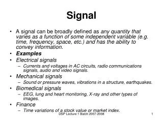
Signal. A signal can be broadly defined as any quantity that varies as a function of some independent variable (e.g. time, frequency, space, etc.) and has the ability to convey information. Examples Electrical signals

Signal
E N D
Presentation Transcript
Signal • A signal can be broadly defined as any quantity that varies as a function of some independent variable (e.g. time, frequency, space, etc.) and has the ability to convey information. • Examples • Electrical signals • Currents and voltages in AC circuits, radio communications signals, audio and video signals. • Mechanical signals • Sound or pressure waves, vibrations in a structure, earthquakes. • Biomedical signals • EEG, lung and heart monitoring, X-ray and other types of images. • Finance • Time variations of a stock value or market index. DSP Lecture 1 Batch 2007-2008
Classification of Signals 1. Real-valued vs. Complex-valued Signals • The value of signal can be real or complex. If a signal assumes real values throughout, then it’s regarded as a real-valued signal. E.g. electric power for residential use (real signal) vs. electric power for industrial use (complex signal) 2. Scalar vs. Vector (Multi-channel) Signals • Sometimes several measurements or sources occur simultaneously. This leads to a multi-channel signal, represented as a vector of signals. Such signals are represented in terms of vectors: • E.g. blood pressure signal (scalar or single-channel) signal vs. 3-channel ECG signal (vector signal) DSP Lecture 1 Batch 2007-2008
Classification of Signals 3. One-Dimensional vs. Multi-Dimensional Signals • An M-dimensional signal is a function of M variables. • Speech is an example of 1-D signal • Image is an example of 2-D signal I(x, y) • “Black-&White” Video is an example of 3-D signal I(x, y, t) • Color video is an example of 3-channel, 3-D signal 4. Deterministic vs. Random Signals • A deterministic signal is predictable and can be represented with an explicit mathematical expression. E.g. test signals. A random signal is unpredictable and must be represented with statistical models. E.g. signal corrupted by noise DSP Lecture 1 Batch 2007-2008
Classification of Signals 5. Continuous-Time (CT) vs. Discrete-Time (DT) Signals • CT signals are defined for every value of time e.g. temperature at any given time. • DT signals are defined only at specific instances of time e.g. audio signal on a CD ROM • DT signals are only defined at the sampling point, they are undefined between samples (the value is not zero). 6. Continuous-Valued (CV) vs. Discrete-Valued (DV) Signals • Amount of current drawn by a device (CV) • Ranking of a school (DV) DSP Lecture 1 Batch 2007-2008
On the basis of continuous or discrete nature of dependent/independent variable, a useful classification of signals can be given as: • CT & CV: analog signal e.g. temperature, speech, etc DSP Lecture 1 Batch 2007-2008
CT & CV: analog signal e.g. temperature, speech, etc • CT & DV: any quantized signal e.g. population • DT & CV: sampled signal e.g. daily average wind speed • DT & DV: sampled and quantized signal. Also known as digital signal. Any signal processed by a computer (or any digital device) must be of this type. e.g. audio/video CD DSP Lecture 1 Batch 2007-2008
When the samples are equally spaced, (i.e. with uniform sampling) where, Fs is the sampling rate or sampling frequency. Given an analog signal xa(t), the corresponding DT version obtained at the sampling rate of Fs is defined as: DSP Lecture 1 Batch 2007-2008
digital signal digital signal analog signal A/D DSP D/A analog signal Digital Signal Processing • Digital Signal Processing is defined as the mathematical and algorithmic manipulation of digital signals in order to extract the most relevant and pertinent information that is carried by the signal. • Basic Components of a DSP System DSP Lecture 1 Batch 2007-2008
The analog-to-digital (A/D) converter transforms the analog signal at the system input into a digital signal. • The sampler acts like a switch, that stays closed for an infinitesimally small amount of time. It takes samples from the continuous time signal. • The resolution or step size in the quantization process can be defined as where L is the number of quantization levels. DSP Lecture 1 Batch 2007-2008
The quantization introduces a quantization error eq(n) illustrated in the diagram shown below: • eq(n) = x(n) – xq(n) • The digital signal processor (the central block) performs the desired operations on the digital signal and produces a corresponding output also in digital form. DSP Lecture 1 Batch 2007-2008
Implementation The operations performed by the digital signal processor can usually be described by means of an algorithm, on which its implementation is based. • The implementation of the digital system can take different forms: • Hardwired in which dedicated digital hardware components are specially configured to accomplish the desired processing task. • Software in which the desired operations are executed via a programmable digital signal processor (PDSP) or a general computer programmed to this end. • The following distinctions are also important: • Real-time system: the computing associated to each sampling interval can be accomplished in a time ≤ the sampling interval. • Off-line system: A non real-time system which operates on stored digital signals. This requires the use of external data storage units. DSP Lecture 1 Batch 2007-2008
Advantages of DSP • More flexible • System characteristics can easily be changed by programming without modification in hardware. Products can be distributed/sold and updated via Internet. • More accurate • Any level of accuracy can be obtained by use of appropriate number of bits. • Higher performance • Efficient implementation of fast algorithms and matrix-based processing • Easier to mass produce • Advantage can be taken of the availability of advanced semiconductor VLSI technology. • Easier to design DSP Lecture 1 Batch 2007-2008
Advantages of DSP • More deterministic and reproducible – less sensitive to component values, etc. • The characteristics of the system will not drift with temperature or ageing • Many things that cannot be done in analog domain can be done digitally • Allows multiplexing, time sharing, multichannel processing, adaptive filtering • Easy to cascade, no loading /drift effects, signals can be stored indefinitely w/o loss of fidelity. On the other hand, stored analog signals deteriorate quickly as the time progresses and cannot be recovered in their original form. • Allows processing of very low frequency signals (or any arbitrary transfer function), which requires impractical component values in analog world, such as those occurring in seismic applications, where inductors and capacitors needed for analog signal processing would be physically very large in size. DSP Lecture 1 Batch 2007-2008
Drawbacks • A digital signal processing system can be slower on account of the overhead introduced by the ADC and DAC conversion. • Increased system complexity because of the need for the additional pre- and post-processing devices such ADC and DAC converters and their associated filters. • Consumes more power. Yet, the advantages far outweigh the disadvantages. Today, most continuous time signals are in fact processed in discrete time using digital signal processors. DSP Lecture 1 Batch 2007-2008
Nature of Processing What kind of processing is done by the digital signal processor? This depends on the area of application: • Communication – Modulation and demodulation • Signal Security – Encryption and decryption • Data Compression – Reduce space/computation required to store/process data • Signal Denoising – Filtering for noise reduction • Image Processing – Image denoising, enhancement, reconstruction • Each of the above can be expressed as a mathematical operation performed on the signal. DSP is then the system that performs this operation. Filtering • This is by far the most commonly used DSP operation It refers to deliberately changing the frequency content of the signal, typically, by removing certain frequencies from the signals. E.g.: • For denoising applications, the (frequency) filter removes those frequencies in the signal that correspond to noise • In communications applications, filtering is used to focus that part of the spectrum that is of interest, that is, the part that carries the information. DSP Lecture 1 Batch 2007-2008
Why Should I Study DSP? • It’s a compulsory course. . . • It has numerous real world applications • Image processing • pattern recognition, robotic vision, image enhancement, facsimile, satellite weather map, animation • Instrumentation and control • spectrum analysis, position and rate control, noise reduction, data compression • Speech and audio • speech recognition, speech synthesis, text to speech, digital audio, equalization • Military • secure communication, radar processing, sonar processing, missile guidance • Telecommunications • echo cancellation, adaptive equalization, spread spectrum, video conferencing, data communication • Biomedical • patient monitoring, scanners, EEG brain mappers, ECG analysis, X-ray storage and enhancement • The number of new applications and improvements to the existing applications will continue to grow at a very rapid rate in the future. DSP Lecture 1 Batch 2007-2008
A Bit of History • Before 1950, signal processing was done with analog circuits. • In 1950s, people began to use digital computers in signal processing to simulate the performance before actually implementing the circuits. DSP couldn’t be done in real-time due to technology constraints. • In 1965, Cooley and Tukey proposed their Fast Fourier transform (FFT) algorithm (to be discussed later in the course), which significantly increased the efficiency of DSP The first major development of DSP. • By the mid-1980s, integrated circuit technology had advanced to the level to make fast microprocessors, which enabled DSP to be done in real-time the second major development of DSP. DSP Lecture 1 Batch 2007-2008


![[Unix Programming] Signal and Signal Processing](https://cdn3.slideserve.com/5708599/unix-programming-signal-and-signal-processing-dt.jpg)