Download
1 / 64
650 likes | 896 Vues
Chapter 5. Estimation of Model Parameters Using Least Squares. 5.1 Introduction 5.2 Regression analysis 5.3 Simple OLS regression 5.4 Multiple OLS regression 5.5 Assumptions and sources of error during OLS 5.6 Model residual analysis 5.7 Other OLS parameter estimation methods

E N D
Chapter 5. Estimation of Model Parameters Using Least Squares 5.1 Introduction 5.2 Regression analysis 5.3 Simple OLS regression 5.4 Multiple OLS regression 5.5 Assumptions and sources of error during OLS 5.6 Model residual analysis 5.7 Other OLS parameter estimation methods 5.8 Case study example: Effect of refrigerant additive on chiller performance Chap 5-Data Analysis Book-Reddy
5.1 Introduction A model is a relation between the variation of: • one variable (called the dependent or response variable) • Against other variables (called independent or regressor variables). If observations (or data) are taken of both response and regressor variables under various sets of conditions, one can build a mathematical model from this information which can then be used as a predictive tool under different sets of conditions. How to analyze the relationships among variables and determine a (if not “the”) optimal relation, falls under the realm of regression model building or regression analysis. Chap 5-Data Analysis Book-Reddy
Let us first limit ourselves to models linear in the parameters • Why “squared deviations” • Why not “absolute deviations” • Why only deviations in y variable Chap 5-Data Analysis Book-Reddy
Fig. 5.4 The value of regression in reducing unexplained variation in the response variable as illustrated by using a single observed point. The total variation from the mean of the response variable is partitioned into two portions: one that is explained by the regression model and the other which is the unexplained deviation, also referred to as model residual Chap 5-Data Analysis Book-Reddy
y = a + b.x Fig. 5.2 Conceptual illustration of how regression explains or reduces unexplained variation in the response variable . It is important to note that the variation in the response variable is taken with reference to its mean value SSR SSE Note that the slope parameter b explains the variation in y due to that in x. It does not necessarily follow that this parameter accounts for MORE of the observed absolute magnitude in y than does the intercept parameter term a Chap 5-Data Analysis Book-Reddy
Fig. 5.5(b) Plot of observed versus OLS model predicted values of the y variable Chap 5-Data Analysis Book-Reddy
5.3.2 Model Evaluation p p p=2 Chap 5-Data Analysis Book-Reddy
p p Hence, a CV value of say 12% implies that the root mean value of the unexplained variation in the dependent variable y is 12% of the mean value of y. Chap 5-Data Analysis Book-Reddy
Internal Prediction Error p Chap 5-Data Analysis Book-Reddy
p Some texts state that the data set should be at least 5-8 times larger than the number of model parameters to be identified. In case of short data sets, OLS may not yield robust estimates of model uncertainty and resampling methods are advocated Chap 5-Data Analysis Book-Reddy
Cross Validation to Avoid Over-Fitting - Danger of “overfitting”, i.e., the model also fits part of the noise in the data along with the system behavior. - In such cases, the model is likely to have poor predictive ability • Cross validation involves: • Randomly partition the data set into two (say in proportion of 80/20), • Use the 80% portion of the data to develop the model, calculate the internal predictive indices CV and NMBE • Use the 20% portion of the data and predict the y values using the already identified model, and finally calculate the external or simulation indices CV and NMBE. • Competing models can then be compared, and a selection made, based on both the internal and external predictive indices. • The simulation indices will generally be poorer than the internal predictive indices; larger discrepancies are suggestive of greater over-fitting, and vice versa. • Note, however, that though the same equations are used to compute the CV and NMBE indices, the degrees of freedom (df) are different. - df=n-p for computing the internal predictive errors where n is the number of observations used for model building, - df=m for computing the external indices where m is the number of observations in the cross-validation set. Chap 5-Data Analysis Book-Reddy
5.3.3 Inferences on regression coefficients and model significance SSR/(p-1) SSE/(n-p) p p- Chap 5-Data Analysis Book-Reddy
5.3.4 Model prediction uncertainty Chap 5-Data Analysis Book-Reddy
5.4 Multiple OLS regression Fig. 5.7 General shape of regression curves Chap 5-Data Analysis Book-Reddy
5.4.1 Higher Order Linear Models Chap 5-Data Analysis Book-Reddy
(a) non-interacting (b) interacting Fig. 5.8 Plots illustrating the effect of interaction among the regressor variables Chap 5-Data Analysis Book-Reddy
5.4.2 Matrix formulation Chap 5-Data Analysis Book-Reddy
5.4.3 OLS parameter identification Chap 5-Data Analysis Book-Reddy
Example 5.4.1. Part load performance of fans (and pumps) Chap 5-Data Analysis Book-Reddy
Independent variable matrix X (b) The results of the regression : Goodness-of-fit R2 = 99.9%, Adjusted R2 = 99.9%, RMSE = 0.009246 Mean absolute error (MAD) = 0.00584. The equation of the fitted model is FFLP = -0.0204762 + 0.179221*PLR + 0.850649*PLR2 Fig. 5.9 Plot of fitted model with 95% CL and 95% PL bands Degrees of freedom for sum of squares of regression model is d.f.=p-1 “ error or residual = n-p “ total =n-1 Number of observations n=9 Chap 5-Data Analysis Book-Reddy
Example 5.4.2. Model for solubility of oxygen in water in (mg/L) at 1 atm pressure for different temperatures and different chloride concentrations in (mg/L). (a) Plot the data and formulate two different models to be evaluated (b) Evaluate both models and identify the better one. (c) Report pertinent statistics for model parameters and overall model fit. Fig. 5.10(a) Plot of data One notes that the series of plots are slightly non-linear but parallel suggesting a higher order model without interaction terms. Hence, first order and second order polynomial models without interaction are logical models to investigate. Chap 5-Data Analysis Book-Reddy
Analysis of the first order without interaction term: R2 = 96.83 %, Adjusted R2 = 96.57%, RMSE = 0.41318 F-ratio=382 Fig. 5.10 (b) Residual pattern for the first order model (b2) Analysis of second order model without interaction term: R2 = 99.26 %, Adjusted R2 = 99.13%, • RMSE = 0.20864 F-ratio=767 Fig. 5.10(c) Residual pattern for the second order Chap 5-Data Analysis Book-Reddy
5.4.4 Partial correlation coefficients • Concept of simple correlation coefficient between two variables can be extended to a MLR model • Since regressors are often “somewhat” correlated- partial correlation coefficients. This allows the linear influence of x2 to be removed from both y and x1, thereby enabling the partial correlation coefficient to describe only the effect of x1 on y which is not accounted for by the other variables in the model. This concept plays a major role in the process of stepwise model identification Chap 5-Data Analysis Book-Reddy
5.5 Assumptions and sources of error during OLS parameter estimation No statistical assumptions are used to obtain the OLS estimators for the model coefficients. When nothing is known regarding measurement errors, OLS is often the best choice for estimating the parameters. However, in order to make statistical statements about these estimators and the model predictions, it is necessary to acquire information regarding the measurement errors. Ideally, one would like the error terms - to be normally distributed, - without serial correlation, • constant variance. • If error terms do not have zero mean or • if regressors are correlated with the errors • or if the regressor measurement errors are large Violations may lead to distorted estimates of the standard errors, confidence intervals, and statistical tests. In addition, the regression model will suffer from BIASED model coefficients Chap 5-Data Analysis Book-Reddy
5.6 Model residual analysis 5.6.1 Detection of ill-conditioned model residual behavior- VERY IMPORTANT (provides insights into model mis-specification) an assessment of the model should be done to determine whether the OLS assumptions are met, otherwise the model is likely to be deficient or mis-specified, and yield misleading results Fig. 5.12 Effect of omitting an important variable. The residuals can be separated into two distinct groups Fig. 5.13 Presence of outliers. Data should be checked and/or robust regression used instead of OLS Chap 5-Data Analysis Book-Reddy
Fig. 5.14 Need for log transformation. Residuals with bow shape and increased variability (i.e., error increases as the response variable y increases) Fig. 5.15 Reformulate model to include higher order. Bow-shaped residuals suggest Fig. 5.16 Presence of serial correlation Pattern in the residuals when plotted in the sequence the data was collected. Chap 5-Data Analysis Book-Reddy
Problems associated with model underfitting and overfitting are usually the result of a failure to identify the non-random pattern in time series data. Fig. 5.17 Plot of the data (x,y) with the fitted lines for four data sets. The models have identical R2 and t-statistics but only the first model is a realistic model Underfitting does not capture enough of the variation in the response variable which the corresponding set of regressor variables can possibly explain Underfit Good Overfitting implies capturing randomness in the model, i.e., attempting to fit the noise in the data. One point has undue influence Chap 5-Data Analysis Book-Reddy
SERIAL CORRELATION- Durbin-Watson Statistics for checking white noise of adjacent residuals If the model underfits, DW < 2 and DW>2 for an overfitted model, the limiting range being 0 to 4. Tables are available for approximate significance tests with different numbers of regressor variables and number of data points (for n=20 and p =3, dL= 1.0 and dU = 1.68) • Table A13 assembles lower and upper critical values of DW statistics to test autocorrelation at the (2x0.05) significance level. Frame the null hypothesis as correlation coefficient=0) • Null hypothesis can be rejected if DW < dL OR 4-DW<dL, i.e. DW is significant • Null hypothesis cannot be rejected if DW > dU AND 4-DW>dU, i.e. DW is not significant • Otherwise the test is inconclusive Chap 5-Data Analysis Book-Reddy
5.6.2 Leverage and influence data points may or may not have a large impact m Chap 5-Data Analysis Book-Reddy
Fig. 5.18 Common patterns of influential observations 5.6.2 Leverage and influence data points Adverse effect Chap 5-Data Analysis Book-Reddy
5.6.2 Leverage and influence data points Chap 5-Data Analysis Book-Reddy
(b) (b) Chap 5-Data Analysis Book-Reddy
Example 5.6.2 Example of variable transformation to remedy improper residual behavior. Data from 27 departments in a university with y as the number of faculty and staff and x the number of students. Chap 5-Data Analysis Book-Reddy
Fig. 5.21 Type of heteroscedastic model residual behavior which arises when errors are proportional to the magnitude of the x variable Ba Basic concept of WLS is to assign different weights to different points According to a certain scheme such that we minimize: Chap 5-Data Analysis Book-Reddy
Example 5.6.3 Example of weighted regression for replicate measurements (laboratory experiment) • Fig. 5.22 (a) Data set and OLS regression line of observations with nonconstant variance and replicated observations in x • Fig. 5.22 (b) Residuals of a simple linear OLS model fit (Eq.5.49a) Chap 5-Data Analysis Book-Reddy
Residuals of simple OLS are strongly heteroscadastic- OLS has misleading uncertainty bands even though the predictions are unbiased Partition the x range into discrete regions Fig. 5.22 (c) Residuals of a second order polynomial OLS fit to the mean x and mean square error (MSE) of the replicate values (Eq. 5.49b) Chap 5-Data Analysis Book-Reddy
(b) (c) Chap 5-Data Analysis Book-Reddy
(d) 5.46 (d) Fig. 5.22 (d) Residuals of the weighted regression model (Eq.5.49c) Chap 5-Data Analysis Book-Reddy
5.6.4 Serially correlated residuals Two different types of autocorrelation: pure autocorrelation and model-misspecification Note that the CO transform is inadequate in cases of model mis-specification and/or seasonal operational changes. Chap 5-Data Analysis Book-Reddy
H T T Fig. 5.23 Chap 5-Data Analysis Book-Reddy
Fig. 5.24 Improvement in residual behavior for a model of hourly energy use of a variable air volume HVAC system in a commercial building as influential regressors are incrementally added to the model 5.6.5 Dealing with misspecified models Chap 5-Data Analysis Book-Reddy
5.7 Other OLS parameter estimation methods 5.7.1 Zero-intercept models Sometimes the physics of the system dictates that the regression line pass through the origin. -Interpretation of R2 not the same as for the model with an intercept, • For the no-intercept case, the R2 value explains the percentage variation of the response variable about the origin explained by that of the regressor variable. 5.7.2 Indicator variables for local piecewise models- spline fits • Very important class of functions, described in numerical analysis textbooks in the framework of interpolation, which allow distinct functions to be used over different ranges while maintaining continuity in the function • They are extremely flexible functions in that they allow a wide range of locally different behavior to be captured within one elegant functional framework. • Thus, a globally nonlinear function can be decomposed into simpler local patterns. Chap 5-Data Analysis Book-Reddy