Download
1 / 47
470 likes | 610 Vues
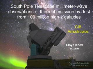
The South Pole Telescope (SPT) provides significant insights into the cosmic infrared background (CIB) by observing millimeter-wave thermal emissions from dust in approximately 100 million high-redshift galaxies. These measurements are crucial for understanding the history of star formation in the universe. The SPT, with its fine-scale anisotropy measurement capabilities, enables in-depth studies of dusty star-forming galaxies and their connection to dark matter. This research contributes valuable data towards modeling star formation and structure growth across cosmic time.

E N D
South Pole Telescope millimeter-wave observations of thermal emission by dust from 100 million high-z galaxies Lloyd Knox UC Davis CIB Anisotropies Photo credit: Keith Vanderlinde SPT 2nd season winter-over
Anisotropies in the CIB are sensitive to the entire history of star formation in the Universe Scientific Motivation I Image: WMAP (slightly hacked by J. Vieira)
Where There’s Star Formation, There’s Dust • Standard lore: Dust forms in cold envelopes of evolved stars and in ejecta of supernovae • Dust also facilitates the cooling necessary for star formation
Optical Properties of Dust Jessberger et al. (2001) Full-sky 94 GHz intensity map Absorbs light at wavelengths smaller than the grain size Radiates thermally at longer wavelengths
Half of background light from stars is reprocessed by dust Dole et al. 2006 CIB Brightness = 24 nW/m2/sr
Simple Model of Dust Emission 34 K grey body spectrum
Rest frequency from z = 1 to z = 5 34 K grey body spectrum
SPT Bands Hall et al. (2010) Dimming redshifting Object of same luminosity gets brighter when moved from z=1 to z=5
Sub-mm magic RS comment
n(z) for SMGs Dye et al 2009 250, 350, 500 um selected 850 um selected 10
z-independent brightness, but bulk of them are very faint • To study in great numbers we need to study them in the confusion limit. • Intensity = s S2 dN/dS d(lnS) • Data points are from SPT (Vieira et al. 2010) DSFG = ? Figures by Nicholas Hall Number density = s S dN/dS (dlnS)
z-independent brightness, but bulk of them are very faint • To study in great numbers we need to study them in the confusion limit. • Intensity = s S2 dN/dS d(lnS) • Data points are from SPT (Vieira et al. 2010) DSFG = Dusty star-forming galaxy Figures by Nicholas Hall Number density = sSdN/dS (dlnS)
Angular power spectra sensitive to relation between dark matter and star formation history • To study in great numbers we need to study them in the confusion limit. • Can measure angular power spectrum of diffuse background, with shape and amplitude dependent on relation of star formation history to dark matter density history. • The latter we can calculate well from first principles. Figures by Nicholas Hall
Outline • Measurement in the confusion limit with SPT*. • Modeling the signals inferred from SPT, BLAST and Spitzer data. • Future observational prospects. • Future modeling challenges. *Many slides in this part from J. Vieira
The South Pole Telescope (SPT) The SPT • An experiment optimized for fine-scale anisotropy measurements of the CMB • Dedicated 10-m telescope at the South Pole • Background-limited 960-element mm camera • Science Goals: • Mass-limited SZ survey of galaxy clusters • study growth of structure, dark energy equation of state • Fine-scale CMB temperature anisotropies • SZ power spectrum to measure σ8 • mm sources • dusty star forming galaxies • AGN • Other rare objects • NEXT: Polarization Funded by NSF
The South Pole Telescope (SPT) Sub-millimeter Wavelength Telescope: • 10 meter telescope ⇒ 1’ FWHM beam at 1.4 mm • Clean and simple optical design to minimize systematics • Off-axis Gregorian optics design for clear aperture • Three levels of sidelobe mitigation: • under-illuminated primary • Co-moving ground shield • cold (10K) secondary • 20 micron RMS surface accuracy (good up to ~ 450 um window) • 1 arc-second relative pointing ⇒ <3" RMS absolute pointing • Fast scanning (up to 4 deg/sec in azimuth) ⇒ no chopping 1st Generation Camera: • 1 sq. deg FOV ⇒ good for surveys, bad for pointed observations • 960 TES coupled spiderweb bolometers read out with SQUIDS and fMUXed • Modular focal plane observes simultaneously in 3 bands at 1.4, 2.0, 3.2 mm with 1.0, 1.5, 2.0 fλ pixel spacing • Closed cycle He cryogenics
SPT Team February 2007 Collaboration
Survey Fields Completed 23hr 5hr30 • In 2008 mapped ~180 deg2 around 5hr and 23hrs to 18 uK/arcmin2 pixel. In 2009 we mapped ~ 550 deg2 to the same depth. • BCS overlap and Magellan follow-up for optical confirmation and photo-z’s. • Full survey will be ~2000 square degrees. Field used for recent results
Zoom in on 2 mm map ~ 4 deg2 of actual data
Zoom in on 2 mm map ~ 4 deg2 of actual data ~15-sigma SZ cluster detection All these “large-scale” fluctuations are primary CMB. Lots of bright emissive sources
Source Count Data points are from SPT(Vieira et al. 2010) DSFG = Dusty Star-Forming Galaxy ULIRG/DSFG model modified from Negrello et al. (2007) Radio galaxy model is from de Zotti et al. (2005) Figure is from Hall et al. (2010) ClPoisson = s S3 dN/dS d(lnS) Data points from counting point sources
Auto and Cross-Frequency Power Spectra: Data at l > 2000 (Hall et al. 2010) Total observed signal Need to develop model for CIB signal in these data
Auto and Cross-Frequency Power Spectra: Data and Model at l > 2000 (Hall et al. 2010) Total observed signal poisson term due to sources at S/N < 5 Best-fit tSZ from L10 Best-fit DSFG-clustering term Assumed kSZ
= comoving distance Scale factor Single-SED Model Dust emissivity index and temperature * Fiducial Model: Td = 34K, = 2, zc = 2, z = 2 Hall et al. (2010) Knox et al. (2001) *Planck function modified to power-law decline on Wien side with “mid-IR” index
Redshift distribution of mean for Lagache, Dole and Puget (2005) model and Hall et al. (2010) single-SED model
Auto and Cross-Frequency Power Spectra: Data and Model at l > 2000 (Hall et al. 2010) Total observed signal poisson term due to sources at S/N < 5 Best-fit tSZ from L10 Best-fit DSFG-clustering term Assumed kSZ
BLAST: Viero et al. (2009), Spitzer: Lagache et al. (2007) Spectrum of Poisson Power • Weak dependence on threshold • LDP model too shallow -- spectrum is steeper than expected at low frequencies • single-SED model is NOT fit to these data
Large 150 to 220 spectral index For S proportional to about = 220 GHz we find = 3.86 § 0.26 from SPT data In RJ limit, = + 2 For Td = 34K and sources at z = 1 (or 2) we get = + 1.7 (or 1.5) Roughly expect for our single-SED model, = 1.38 + = 3.38 Theoretical models calibrated with astronomical and laboratory data suggest ~ 2 (Gordon 1995). Meny et al. (2007) claim effects of long-range disorder in dust can lead to > 2 Silva et al. (1998) models
BLAST: Viero et al. (2009), Spitzer: Lagache et al. (2007) Spectrum of Poisson Power Can get away with lower if assume higher Td or lower z, but then over-predict BLAST and Spitzer power.
Auto and Cross-Frequency Power Spectra: Data and Model at l > 2000 (Hall et al. 2010) Total observed signal poisson term due to sources at S/N < 5 Best-fit tSZ from L10 Best-fit DSFG-clustering term much stronger at 220x220 than 150x220 Assumed kSZ
Clustering amplitudes at theoretically expected levels (RJ) Haiman & Knox (2000)
Clustering amplitudes at expected levels • Mean CIB inferred from FIRAS data • a few arc minutes corresponds to several comoving Mpc • variance in density fluctuations is order unity on Mpc scales • line of sight probes a few hundred independent cells • I/I = b/3000.5 = 0.1 Puget et al. (1996) Fixsen et al. (1998) Reproduces observed clustering power
Outline • Measurement in the confusion limit with SPT*. • Modeling the signals inferred from SPT, BLAST and Spitzer data. • Future observational prospects. • Future modeling challenges. *Many slides in this part from J. Vieira
Clustering power will be measured with high precision by Planck very soon CIB is the dominant source of fluctuation power over large parts of sky, and a large range of angular scales in the highest frequency channels of Planck Knox et al. (2001) Relevant Planck channels: 143, 217, 353, 545, 850 GHz
Precision Measurement Expected from Planck Milky Way Dust • F for FIRB = CIB • Forecast for Planck 545 GHz shown • In addition will have auto and cross-frequency power from 217, 353, 545, 850
Cross-correlation opportunities • CIB anisotropies arise from a broad range in redshifts and therefore have cross correlations with other tracers of large-scale structure • Can reconstruct the lensing potential from the lensed CMB and cross-correlate with CIB Lensing-FIRB cross-power forecast for Planck Song et al. (2003)
Cross-correlate with CMB2! Square of kSZ signal correlates with cosmic shear (Dore et al. 2003) Should also correlate with CIB -- might be first way effect of kSZ is detected
dusty star forming galaxy gas-rich merger AGN dominated phase massive elliptical dust from SN + debris disks Narayanan+2009 Slide from J. Vieira
Another model Righi, Hernandez-Monteagudo & Sunyaev (2008) Righi et al. work out CIB power spectrum predictions associating DSFGs with mergers
Righi et al. predictions SPT detected clustering power at 220 GHz
Phenomenology ripe for development • Merger model of Righi et al. can accommodate data as well as the `light traces (halo) mass’ models. • How do we discriminate? • How do we parameterize the connection between star formation and dark matter evolution to help us interpret the forthcoming high-precision data? • I am working on these questions with Z. Haiman (Columbia) and A. Benson (Caltech)
Lueker et al. 2010 bandpowers from subtraction Ts = 1/(1-0.325) (T150 - 0.325 T220) For subtracting DSFGs (Dusty Star-Forming Galaxies) Best-fit residual DSFG Poisson Power Best-fit tSZ Assumed kSZ Possible Patchy reionization signal (not included in modeling) 46
Summary • CIB offers us a probe of entire history of star formation • From SPT data, we have a first detection of the clustering of CIB at millimeter wavelengths, at expected amplitudes. • A simple model can accommodate frequency dependence of CIB anisotropy from 150 to 1900 GHz (with steep emissivity index) • Observational progress in the confusion limit will be rapid and is driving the development of theoretical modeling to facilitate interpretation • Phenomenology of the CIB is very ripe for further development, so that we can turn the observational signatures into interesting conclusions about the history of star formation in the Universe.