Constraint Satisfaction Problems

Constraint Satisfaction Problems Tuomas Sandholm Carnegie Mellon University Computer Science Department Read Chapter 6 of Russell & Norvig

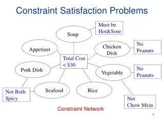
Constraint satisfaction problems (CSPs) • Standard search problem: state is a "black box“ – any data structure that supports successor function and goal test CSP: • state is defined by variablesXi with values from domainDi • goal test is a set of constraints specifying allowable combinations of values for subsets of variables • Simple example of a formal representation language • Allows useful general-purpose algorithms with more power than standard search algorithms

Example: Map-Coloring • VariablesWA, NT, Q, NSW, V, SA, T • DomainsDi = {red,green,blue} • Constraints: adjacent regions must have different colors e.g., WA ≠ NT, or (WA,NT) in {(red,green),(red,blue),(green,red), (green,blue),(blue,red),(blue,green)}

Example: Map-Coloring • Solutions are complete and consistent assignments • E.g., WA = red, NT = green, Q = red, NSW = green,V = red,SA = blue,T = green

Constraint graph • Binary CSP: each constraint relates two variables • Constraint graph: nodes are variables, arcs are constraints

Varieties of CSPs • Discrete variables • finite domains: • n variables, domain size d  O(dn) complete assignments • E.g., Boolean CSPs, incl. Boolean satisfiability (NP-complete) • infinite domains: • integers, strings, etc. • E.g., job scheduling, variables are start/end days for each job • need a constraint language, e.g., StartJob1 + 5 ≤ StartJob3 • Continuous variables • E.g., start/end times for Hubble Space Telescope observations • linear constraints solvable in polynomial time by linear programming (LP)

Varieties of constraints • Unary constraints involve a single variable, • e.g., SA ≠ green • Binary constraints involve pairs of variables, • e.g., SA ≠ WA • Higher-order constraints involve 3 or more variables, • e.g., cryptarithmetic column constraints

Backtracking search • Variable assignments are commutative, i.e., [ WA = red then NT = green ] same as [ NT = green then WA = red ] • => Only need to consider assignments to a single variable at each node • Depth-first search for CSPs with single-variable assignments is called backtracking search • Can solve n-queens for n≈ 25

Backtracking example

Improving backtracking efficiency • General-purpose methods can give huge gains in speed: • Which variable should be assigned next? • In what order should its values be tried? • Can we detect inevitable failure early?

Most constrained variable • Most constrained variable: choose the variable with the fewest legal values • a.k.a. minimum remaining values (MRV) heuristic

Most constraining variable • A good idea is to use it as a tie-breaker among most constrained variables • Most constraining variable: • choose the variable with the most constraints on remaining variables

Least constraining value • Given a variable to assign, choose the least constraining value: • the one that rules out the fewest values in the remaining variables • Combining these heuristics makes 1000 queens feasible

Forward checking • Idea: • Keep track of remaining legal values for unassigned variables • Terminate search when any variable has no legal values

Constraint propagation • Forward checking propagates information from assigned to unassigned variables, but doesn't provide early detection for all failures: • NT and SA cannot both be blue! • Constraint propagation algorithms repeatedly enforce constraints locally…

Arc consistency • Simplest form of propagation makes each arc consistent • X Y is consistent iff for every value x of X there is some allowed y

Arc consistency • Simplest form of propagation makes each arc consistent • X Y is consistent iff for every value x of X there is some allowed y • If X loses a value, neighbors of X need to be rechecked

Arc consistency • Simplest form of propagation makes each arc consistent • X Y is consistent iff for every value x of X there is some allowed y • If X loses a value, neighbors of X need to be rechecked • Arc consistency detects failure earlier than forward checking • Can be run as a preprocessor or after each assignment

Arc consistency algorithm AC-3 • Time complexity: O(#constraints|domain|3) Checking consistency of an arc is O(|domain|2)

k-consistency • A CSP is k-consistent if, for any set of k-1 variables, and for any consistent assignment to those variables, a consistent value can always be assigned to any kth variable • 1-consistency is node consistency • 2-consistency is arc consistency • For binary constraint networks, 3-consistency is the same as path consistency • Getting k-consistency requires time and space exponential in k • Strong k-consistency means k’-consistency for all k’ from 1 to k • Once strong k-consistency for k=#variables has been obtained, solution can be constructed trivially • Tradeoff between propagation and branching • Practitioners usually use strong 2-consistency and less commonly 3-consistency

Other techniques for CSPs • Global constraints • E.g., Alldiff • Bipartite graph with variables on one side, values on the other; only edges that belong to some matching that matches all variables (can be determined in polytime) can belong to a valid assignment • E.g., Atmost(10,P1,P2,P3), i.e., sum of the 3 vars ≤ 10 • Special propagation algorithms • Bounds propagation • E.g., number of people on two flight D1 = [0, 165] and D2 = [0, 385] • Constraint that the total number of people has to be at least 420 • Propagating bounds constraints yields D1 = [35, 165] and D2 = [255, 385] • … • Symmetry breaking

Structured CSPs

Tree-structured CSPs

Algorithm for tree-structured CSPs

Nearly tree-structured CSPs (Finding the minimum cutset is NP-complete.)

Algorithm: solve for all solutions of each subproblem. Then, use the tree-structured algorithm, treating the subproblem solutions as variables for those subproblems. O(ndw+1) where w is the treewidth (= one less than size of largest subproblem) E.g., treewidth of a tree is 1 Finding a tree decomposition of smallest treewidth is NP-complete, but good heuristic methods exists… Every variable in original problem must appear in at least one subproblem If two variables are connected in the original problem, they must appear together (along with the constraint) in at least one subproblem If a variable occurs in two subproblems in the tree, it must appear in every subproblem on the path that connects the two Tree decomposition

State of knowledge on treewidth algorithms • Determining whether treewidth of a given graph is at most k is NP-complete • O(sqrt(log n)) approximation of treewidth in polytime [Feige, Hajiaghayi and Lee 2008] • O(log k) approximation of treewidth in polytime [Amir 2002, Feige, Hajiaghayi and Lee 2008] • When k is any fixed constant, the graphs with treewidth k can be recognized, and a width k tree decomposition can be constructed for them, in linear time [Bodlaender 1996] • There is an algorithm that approximates the treewidth of a graph by a constant factor of 3.66, but it takes time that is exponential in the treewidth [Amir 2002] • Constant approximation in polytime is an important open question

An example CSP: satisfiability

p1 clause T p2 F T F p3 p4 Davis-Putnam-Logemann-Loveland (DPLL) tree search algorithm E.g. for 3SAT ? s.t. (p1p3p4)  (p1p2p3)  … Backtrack when some clause becomes empty Unit propagation (for variable & value ordering): if some clause only has one literal left, assign that variable the value that satisfies the clause (never need to check the other branch) Boolean Constraint Propagation (BCP): Iteratively apply unit propagation until there is no unit clause available Complete

A helpful observation for the DPLL procedure P1 P2  …  Pn  Q (Horn) is equivalent to (P1  P2  …  Pn)  Q (Horn) is equivalent to P1  P2  …  Pn  Q (Horn clause) Thrm. If a propositional theory consists only of Horn clauses (i.e., clauses that have at most one non-negated variable) and unit propagation does not result in an explicit contradiction (i.e., Pi and Pi for some Pi), then the theory is satisfiable. Proof. On the next page. …so, Davis-Putnam algorithm does not need to branch on variables which only occur in Horn clauses

Proof of the thrm Assume the theory is Horn, and that unit propagation has completed (without contradiction). We can remove all the clauses that were satisfied by the assignments that unit propagation made. From the unsatisfied clauses, we remove the variables that were assigned values by unit propagation. The remaining theory has the following two types of clauses that contain unassigned variables only: P1  P2  …  Pn  Q and P1  P2  …  Pn Each remaining clause has at least two variables (otherwise unit propagation would have applied to the clause). Therefore, each remaining clause has at least one negated variable. Therefore, we can satisfy all remaining clauses by assigning each remaining variable to False.

Variable ordering heuristic for DPLL [Crawford & Auton AAAI-93] Heuristic: Pick a non-negated variable that occurs in a non-Horn (more than 1 non-negated variable) clause with a minimal number of non-negated variables. Motivation: This is effectively a “most constrained first” heuristic if we view each non-Horn clause as a “variable” that has to be satisfied by setting one of its non-negated variables to True. In that view, the branching factor is the number of non-negated variables the clause contains. Q: Why is branching constrained to non-negated variables? A: We can ignore any negated variables in the non-Horn clauses because • whenever any one of the non-negated variables is set to True the clause becomes redundant (satisfied), and • whenever all but one of the non-negated variables is set to False the clause becomes Horn. Variable ordering heuristics can make several orders of magnitude difference in speed.

Constraint learning aka nogood learning aka clause learningused by state-of-the-art SAT solvers • Conflict graph • Nodes are literals • Number in parens shows the search tree level • where that node got decided or implied • Cut 2 gives the first-unique-implication-point (i.e., 1 UIP on reason side) constraint • (v2 or –v4 or –v8 or v17 or -v19). That scheme performs well in practice. • Any cut that separates the conflict from the reasons would give a valid clause. • Which cuts should we use? Should we delete some? • The learned clauses apply to all other parts of the tree as well.

Conflict-directed backjumping Dotted arrows not explored yet x7=0 Failure-driven assertion (not a branching decision): Learned clause is a unit clause under this path, so BCP automatically sets x7=0. x2=0 • Then backjump to the decision level of x3=1, • keeping x3=1 (for now), and • forcing the implied fact x7=0 for that x3=1 branch • WHAT’S THE POINT? A: No need to just backtrack to x2

Classic readings on conflict-directed backjumping, clause learning, and heuristics for SAT • “GRASP: A Search Algorithm for Propositional Satisfiability”, Marques-Silva & Sakallah, IEEE Trans. Computers, C-48, 5:506-521,1999. (Conference version 1996.) • (“Using CSP look-back techniques to solve real world SAT instances”, Bayardo & Schrag, Proc. AAAI, pp. 203-208, 1997) • “Chaff: Engineering an Efficient SAT Solver”, Moskewicz, Madigan, Zhao, Zhang & Malik, 2001 (www.princeton.edu/~chaff/publication/DAC2001v56.pdf) • “BerkMin: A Fast and Robust Sat-Solver”, Goldberg & Novikov, Proc. DATE 2002, pp. 142-149 • See also slides at http://www.princeton.edu/~sharad/CMUSATSeminar.pdf

Generalizing backjumping for CSPs

Basic backjumping in CSPs • Conflict set of a variable: all previously assigned variables connected to that variable by at least one constraint • When the search reaches a variable V with no legal values remaining, backjump to the most recently assigned variable in V’s conflict set • Conflict set is updated while trying to find a legal value for the variable • Vertex C has no legal values left! • The search backjumps to the most recent vertex in its conflict set: • Un-assigns value to B, un-assigns value to A • Retries a new value at A • If no values left at A, backjump to most recent node in its conflict set, et cetera search path Values(A) = {R,B} A Values(B) = {R,B} Values(B) = {B} B C Conflicts(C) = {} Conflicts(C) = {A=R} Values(C) = {R} Values(C) = {} Every branch pruned by basic backjumping is also pruned by forward checking

Conflict-directed backjumping in CSPs • Basic backjumping isn’t very powerful: • Consider the partial assignment {WA=red, NSW=red} • Suppose we set T=red next • Then we assign NT, Q, V, SA • We know no assignment can work for these, so eventually we run out of values for NT • Where to backjump? • Basic backjumping wouldn’t work, i.e., we’d just backtrack to T (because NT doesn’t have a complete conflict set with the preceding assignments: it does have values available) • But we know that NT, Q, V, SA, taken together, failed because of a set of preceding variables, which must be those variables that directly conflict with the four • => Deeper notion of conflict set: it is the set of preceding variables (WA and NSW) that caused NT, together with any subsequent variables, to have no consistent solution • We should backjump to NSW and skip over T. • Conflict-directed backjumping (CBJ): • Let Xj be the current variable, and conf(Xj) its conflict set. We exhaust all values for Xj. • Backjump to the most recently assigned variable in conf(Xj), denoted Xi. • Set conf(Xi) = conf(Xi) conf(Xj) – {Xi} • If we need to backjump from Xi, repeat this process.

Nogood learning in CSPs • Conflict-directed backjumping computes a set of variables and values that, when assigned in unison, creates a conflict • It is usually the case that only a subset of this conflict set is sufficient for causing infeasibility • Idea: Find a small set of variables from the conflict set that causes infeasibility • We can add this as a new constraint to the problem or put it in a dynamic nogood pool • Useful for guiding future search paths away from similar problem (i.e., guaranteed infeasible) areas of the search space • Conflict sets are either local or global: • Global: If this subset of variables have these certain values, the problem is always infeasible • Local: Constraint is only valid for a certain subset of search space

More on conflict-directed backjumping (CBJ) • These are for general CSPs, not SAT specifically: • “Conflict-directed backjumping revisited” by Chen and van Beek, Journal of AI Research, 14, 53-81, 2001: • As the level of local consistency checking (lookahead) is increased, CBJ becomes less helpful • A dynamic variable ordering exists that makes CBJ redundant • Nevertheless, adding CBJ to backtracking search that maintains generalized arc consistency leads to orders of magnitude speed improvement experimentally • “Generalized NoGoods in CSPs” by Katsirelos & Bacchus, National Conference on Artificial Intelligence (AAAI-2005) pages 390-396, 2005 • This paper generalizes the notion of nogoods, and shows that nogood learning (then) can speed up (even non-SAT) CSPs significantly • “An optimal coarse-grained arc consistency algorithm” by Bessiere et al. Artificial Intelligence, 2005 • Fastest CSP solver; uses generalized arc consistence and no CBJ

Random restarts

Random restarts • Sometimes it makes sense to keep restarting the CSP/SAT algorithm, using randomization in variable ordering [see, e.g., work by Carla Gomes et al.] • Avoids the very long run times of unlucky variable ordering • On many problems, yields faster algorithms • Heavy-tailed runtime distribution is a sufficient condition for this • All good complete SAT solvers use random restarts nowadays • Clauses learned can be carried over across restarts • Experiments suggest it does not help on optimization problems (e.g., [Sandholm et al. IJCAI-01, Management Science 2006]) • When to restart? • If there were a known runtime distribution, there would be one optimal restart time (i.e., time between restarts). Denote by R the resulting expected total runtime • In practice the distribution is not known. Luby-Sinclair-Zuckerman [1993] restart scheme (1,1,2,1,1,2,4, 1,1,2,1,1,2,4,8,…) achieves expected runtime  R(192 log(R) + 5) • Useful, and used, in practice • The theorem was derived for independent runs, but here the nogood database (and the upper and lower bounds on the objective in case of optimization) can be carried over from one run to the next

Phase transitions in CSPs

Constraint Satisfaction Problems