Medium Access Control
Medium Access Control. Tanenbaum (Chapter 4) Others References: Walrand J., Communication Networks: A first Course Bertesekas and Gallager, Data Networks . Where in the OSI Reference Model ?. Application. Presentation. Session. Transport. Medium Access Control. Network. Link Layer.

Medium Access Control
E N D
Presentation Transcript
Medium Access Control Tanenbaum (Chapter 4) Others References: Walrand J., Communication Networks: A first Course Bertesekas and Gallager, Data Networks
Where in the OSI Reference Model ? Application Presentation Session Transport Medium Access Control Network Link Layer Data Link Layer Physical Medium Access Control
Why Do We Need a MAC Layer ? • Let us consider different topologies • Point-to-point channel • full duplex • half duplex • Broadcast channel Medium Access Control
Management of Broadcast Channels • Contention free: allocating statically shares of the channel to all stations (by TDM, FDM, or other) • Contention: let stations compete for the ALL channel Servers One server Medium Access Control
Objectives of This Chapter:Establish A Key Result • 1) Efficiency: with heavy load, contention free systems are better than contention systems. • 2) For average delay: contention systems are better than contention free (Whatever is the protocol! ) Introduction to Queueing Theory Medium Access Control
Objectives of This Chapter (cont’d):Establish some Properties • Relationship between a MAC protocol and physical properties of network: • Upperbound on efficiency • Maximum length of medium • Bandwidth • Minimum packet size Medium Access Control
Objectives of This Chapter (cont’d):Techniques of Analysis • Initiate students to the techniques used to analyze the performance of MAC protocols: • Aloha protocol • Slotted Aloha • CSMA • CSMA/CD Medium Access Control
Objective 1: Establish A Key Result on Average Delay Queueing Theory
Introduction to Analytical Modeling L.Kleinrock, “Queueing Systems” R.Jain, “The Art of Computer Systems Performance Analysis” E. Modiano, MIT course on Communications
Packet Switched Networks PS PS PS PS PS PS PS Buffer Packet Switch PS Medium Access Control
Queues Everywhere • Processes waiting for CPU • I/O Disk requests • Network interface card • IP input (output) queues • Events (mouse click, keyboard…) • ……………………… Medium Access Control
Queueing Theory • What creates queues? • Randomness!!! • Used for analyzing network performance • In packet networks, randomness comes from: • random packet arrival • Random packet length • Information of interest: • Delay in buffer (queueing delay) • Buffer size Medium Access Control
Queueing Theory Servers jobs Job Sources Or customers Medium Access Control
A Queueing System A/S/m/B/K/SD • A : Interarrival time of jobs distribution • S : The service time distribution • m : Number of servers • B : Capacity of the system (max # of jobs allowed) • K : population size • SD : Service discipline • Default values B = ∞; K=∞; and Z=FCFS • For A and B • G : General distribution • M : Exponential Distribution (memoryless property) • D : Deterministic Medium Access Control
Example • M/D/2/15/20000/FCFS • Time between arrivals exponentially distributed • Service time constant (no variation) • 2 servers • System capacity is 15 (2 places for currently served + 13 waiting) • Population is 20000 (20000 customers will ever come to the system) • Service discipline is first come first served Medium Access Control
Queueing Models • Model good for • Requests received by Google • Customers waiting in line • Packets waiting to be transmitted over a line • Information of interest • Average number of customers in the system • Average delay experienced by a customer Medium Access Control
Queueing System: Variables of Interest • Mean arrival rate: l • Mean service rate: m (service time per job) • Number of customers in system: n • Waiting time (in queue+service): w Servers jobs Job Sources Or customers Medium Access Control
A Key Result : Little’s Law Arrivals Departure Black Box Mean # in system = Mean arrival rate X mean time spent in system E(n) = l.E(w) Remarks : - Result independent of A/B distributions or SD - Can be applied to all system or part of it - Crowded system long delays Medium Access Control
A Key Result : Little’s LawExample A monitor on an HTTP server showed that the average time to satisfy a request was about 50 milliseconds. The requests arrival rate is 200 requests per second. What should be the buffer size (unit is requests) at the http server For the requests ? Little’s law states E(n) = l. E(w) Here l =200 req/s and E(w) = 0.050 s The expected number of customers in the system is E(n) E(n) = 200 x 0.050 = 10 It would be safe to have a buffer size of 20 Medium Access Control
Arrival Process • Packets arrive according to some random process • There are many stochastic processes. • A nice stochastic process is the Poisson process • Mean arrival rate of l packets per second • Prob(n arrivals during T) = [(l.T)n e-lT]/n! Medium Access Control
Example • The number of phone calls arriving to a switch can be closely modeled as a Poisson process. Suppose that the mean arrival rate is 100 per hour. • What is the probability to receive 10 calls in 6 minutes? T = 0.1 hour, l = 100/h Prob(n arrivals during T) = [(l.T)n e-lT]/n! Prob(10 arrivals during 0.1 h)= (100x0.1)10xe-(100x0.1)/10!=0.12 Prob(10 arrivals during 15 mn) = 0.003 Medium Access Control
InterArrival Times of Poisson Process • This is the time between consecutive arrivals. IA is a continuous random variable • What is its probability distribution function? • Prob(IA <= t) = 1 – Prob(IA > t) • = 1 - Prob(0 arrivals within t) • Prob(0 arrivals during t) = [(l.t)0 e-lt]/0!= e-lt • So, Prob(IA <= t) = 1 - e-lt Medium Access Control
InterArrival Times of Poisson Process (2) • The cumulative distribution function (CDF) is: • Prob(IA <= t) = 1 - e-lt • The probability distribution function is the derivative of CDF, i.e., PDF = l.e-lt • This what is called the exponential distribution • This distribution is largely used to model the service times, time between error losses, .. Medium Access Control
Memoryless Property • Def: A random variable X is said to be without memory, or memoryless, • P(X>s+t|X>t) = P(X>s) for all s, t ≥ 0 • In words: “When I get to the bus station, I am told that the probability that the bus comes within the next 10 minutes is 0.90. After one hour waiting, I am told that the probability that the bus comes within the next 10 minutes is still 0.90 ” • Important result : X is memoryless iff it is exponentially distributed Medium Access Control
More Examples • Suppose that the time to graduate from AU is exponentially distributed with mean 4 years. • Given that a student already spent 3 years at AU, what is the expected remaining time before he graduates? Medium Access Control
Properties of Poisson Process (PP) • Merging of K P.P with mean rate li results in a P.P with mean rate the sum of the li’s. • Splitting (randomly) a P.P with mean rate l with probabilities pi results in P.Ps with mean rates pi. l. l1 Sli l2 li ln p1.l1 p2.l2 l pi.li pn.ln Medium Access Control
Analysis of an M/M/1 Queue • Interarrival exponentially distributed (Memoryless) • Service time exponentially distributed (Memoryless) • One server • Infinite capacity of system • Infinite population • First come, first served Jobs Source Server Medium Access Control
Analysis of an M/M/1 (2) • We are interested in the average number of jobs in the system, the average waiting time in the system, or in the probability to have a given number of customers in the system. • Notations • N(t): number of jobs in system at time t • Pn(t) = Prob{N(t)=n} • Pn = lim t-->∞ Pn(t) • l= arrival rate • m = service rate (service time = 1/ m) Medium Access Control
Markov Chain for M/M/1 System l.d l.d l.d l.d l.d l.d 0 1 2 3 4 5 • Circle i = state i means there are i customers in the system • What is the probability Prob(i,j), i.e, the probability of transition from state i and j? • Prob(j,j+1) = l.d, and Proj(j,j-1) = m.d 1-l.d m.d m.d m.d m.d m.d m.d Medium Access Control
Remarks about M/M/1 • l > m, otherwise the system will be instable • After some time in operation, an M/M/1 gets into some equilibrium. • When in equilibrium l.Pi = m.Pi+1 l l l l l l 0 1 2 3 4 5 m m m m m m l i m Medium Access Control
Determining Pn l l l l l l 0 1 2 3 4 5 m m m m m m l.Po = m.P1 l.P1 = m.P2 ………….. l.Pn = m.Pn+1 P1 = (l\m).P0 P2 = (l\m).P1 ………….. Pn+1 = (l\m).Pn Pn = (l\m)n.P0 Using the equations above and the sum SPi = 1, we can derive Pi’s SPi = S (l\m)i.P0 = P0.S (l\m)i = P0/(1-(l\m)) = P0/(1-r) = 1 P0 =(1-r) Pi = ri.(1-r) Medium Access Control
Mean Queue Length E(N) = r/(1-r)r =l/m is the traffic intensity • The average number of customers in the system is E(N) • E(N) = Si.ri.(1-r) = r/(1-r) • E(N) = (1-r).Si.ri • E(N) = r/(1-r) • E(N) = l/(m-l) Medium Access Control
Mean Waiting Time E(W) = 1/(1-r)m • What is the average time in the system? (queueing delay + service time) • We use Little’s formula: E(N) = l.E(W) Medium Access Control
Prob{Server is busy} ? Medium Access Control
Prob{Server is idle} ? Medium Access Control
Analysis of M/M/m (m=3) l l l l l l 0 1 2 3 4 5 m 2m 3m 3m 3m 3m lPo = mP1 lP1 = 2mP2 ………….. lPn = 3mPn+1 Using the equations above and the sum Spi = 1, we can derive Pi’s Medium Access Control
Example • Comparison source partition vs global FCFS • Let the system have n sources and m servers.Jobs generate at each source as P.P with rate l • Job’s computation time is exponentially distributed 1/m • Source partition is m M/M/1 while global FCFS may be viewed as M/M/m with Arrival rate n.l. Medium Access Control
A Fundamental Result In Queueing Theory • One powerful server for all is better than one weak server for each one ! • Why ? Better utilization, as a dedicated channel may stay IDLE. One server Medium Access Control
Analysis of MAC Protocols Read Tanenbaum Chapter 4 Key sections (Intro, 4.1, 4.2.1,4.2.2, 4.3)
Multiple Access Protocols • Competing stations (possible collisions) • Aloha • Slotted Aloha • CSMA • CSMA/CD • Collision-free • Bit-map protocol • Binary countdown • Limited contention • Adaptive tree walk protocol Medium Access Control
Pure Aloha • Designed by Abramson (wireless) • A station emits whenever it has something to send • If other station emits, a collision happens • If collision, frame must be resent • Best possible utilization at high load 18% Medium Access Control
Analysis of Pure Aloha • Assume infinite population of users • Let Tr=time to trasmit a frame (“frame time”) • The population generates a traffic that is Poisson with mean N per “frame time” (new frames) • Since there are also retransmissions, the total traffic generated is Poisson with mean G • What is the throughput S? • S = G.Po where Po is the probability that a frame does not suffer a collision Medium Access Control
Analysis of Pure Aloha (2) (Example) • Suppose that the bandwidth is 10 Mbps, and packet size is 1500 bytes • Tr= 1500.8/10 Mbps = 1.2 ms • Possible values for N (mean number of frames generated per time frame): between 0 and 1 • Values for generated traffic (G > N) • No retransmissions at all G = N • Low load G~N • High load G > N • Po will be higher at low load Medium Access Control
Analysis of Pure Aloha (3) • What is the probability to generate k frames during a “frame time”? • Prob(k arrivals during 1) = [(G.1)k e-G.1]/k! (page 20) • What is the probability Po that that a frame does not suffer a collision? Tr t0 t0+Tr t0+2Tr t0+3Tr Medium Access Control
Analysis of Pure Aloha (4) • Po is the probability that ZERO frame is generated during the vulnerable period • Po = Prob(0 arrivals during 2) = • = [(G.2)0 e-G.2]/0! • Po = e-G.2 • S = G.Po = G.e-G.2 (When is S maximum?) • The maximum throughput S is 1/(2.e) = 18.4% Tr t0 t0+Tr t0+2Tr t0+3Tr Medium Access Control
Slotted Aloha • Designed by Roberts (wireless) • Requires synchronization and division of time in discrete slots • A station emits whenever it has something to send AND must wait for beginning of slot • Best possible utilization at high load 37% t t0 t0+t t0+2t t0+3t Medium Access Control
Analysis of Slotted Aloha (2) • The key: slotted time reduces the vulnerable period to Tr (instead of 2Tr). • Po = Prob(0 arrivals during 1) = • = [(G.1)0 e-G.1]/0! • Po = e-G.1 • S = G.Po = G.e-G (When is S maximum?) • The maximum throughput S is 1/e = 36% • Exercise: derive the average number of transmissions of one frame before being successful. t t0 t0+t t0+2t t0+3t Medium Access Control
Carrier Sense Multiple AccessCSMA • Designed by Metcalfe, analyzed by Kleinrock and Tobaggi • A station listens to the channel before sending. • If channel busy, wait until it becomes idle • When channel free, send with probability 1 • Are collisions still possible? Medium Access Control
Collisions with CSMA • Key: signal takes time tp to propagate • Problem 1: If two stations are listening to grab the channel… • Problem 2: If S1 starts transmitting, S2 may well send during tp. • Problem 3: S1 is not aware of the collision Sender S1 Sender S2 tp Medium Access Control
Solving Problem 1: p-persistent CSMA • 1-persistent: after collision, waits a random time and starts over (slide 48) • Non persistent: if channel busy, the station does not keep listening, but rather waits for a random time before listening again. • p-persistent: for slotted, if idle, send with probability p, otherwise defers to next slot • Much better utilization than Aloha, may go beyond 95%. Medium Access Control