Download
1 / 64
650 likes | 694 Vues
Discover the fundamentals and applications of SAXS in studying molecular structures, biological macromolecules, and more. Learn about interpreting scattering curves, estimating molecular size, and obtaining structural parameters from SAXS data.

E N D
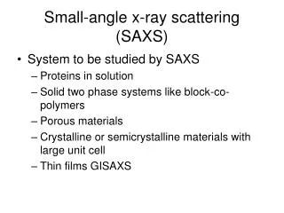
What is SAXS? • Small Angle X-ray Scattering • Scattering proportional to l/Molecular size • Typical x-ray wavelengths ~ 0.1 nm • Typical molecular dimensions 1 -100 nm • Scattering angles are small • 0-2o historically. • Now 0-15o rangeis of increasing experimental interest
Why SAXS ? • Atomic level structures from crystallography or NMR “gold standard” for structural inferences • Crystallography, by definition, studies static structures • Most things crystallize only under rather specific, artificial conditions • Kinetics of molecular interactions frequently of interest • SAXS can provide useful, although limited, information on relatively fast time scales
Why not visible light? • Diffraction effects limit to ~ /50 (5) • i.e. 14 nm visible light vs 1- 2nm RG for small proteins • Water absorbs many wavelengths of light strongly • 0.2 < < 160 nm experimentally inaccessible
What is SAXS Used for? • Estimating sizes of particulates • Interactions in fluids • Sizes of micelles etc in emulsions • Size distributions of subcomponents in materials • Structure and dynamics of biological macromolecules
SAXS and Biological Macro-molecules • How well does the crystal structure represents the native structure in solution? • Can we get even some structural from large proportion of macro-molecules that do not crystallize? • How can we test hypotheses concerning large scale structural changes on ligand binding etc. in solution • SAXS can frequently provide enough information for such studies • May even be possible to deduce protein fold solely from SAXS data
e- e- e- e- e- e- Scattering from Molecules destructive interference Molecules are much larger than the wavelength (~0.1 nm) used => scattered photons will differ in phase from different parts of molecule Observed intensity spherically averaged due to molecular tumbling Constructive interference
Intensity in SAXS Experiments: • Sum over all scatterers (electrons) in molecule to get structure factor (in units of scattering of 1 electron) F(q) = i e i q • ri • Intensity is square (complex conjugate) of structure factor I(q) = F F* = ji e iq •ri,j • Isotropic, so spherical average ( is rotation angle relative to q) I(q) = ji e iq • ri,j sin d • Debye Eq. <I>(q) = ij sin q ri,j/ q ri,j where q = 4sin q/l = 2/d
In Scattering Experiments, Particles are Randomly Oriented • Intensity is spherically averaged • Phase information lost • Low information content fundamental difficulty with SAXS • Only a few, but frequently very useful, structural parameters can be unambiguously obtained.
Structural Parameters Obtainable from SAXS • Molecular weight* • Molecular volume* • Radius of gyration (Rg) • Distance distribution function p( r ) • Various derived parameters such as longest cord from p ( r ) • * requires absolute (or calibrated) intensity information
200 cm 30 cm Experimental Geometry Collimated X-ray beam Sample in 1 mm capillary Backstop “long camera ~1o Detector short camera ~ 15o
The data: Shadow of lead beam stop 2-D data needs to be radially integrated to produce 1-D plots of intensity vs q
Scattering Curves From Cytochrome C Red line = sample +buffer Blue = buffer only Black = difference I ln I q nm-1
What does this look like for a typical protein ? Since a Fourier transform, inverse relationship: Large features at small q Small features at large q Globular size Domain folds 2o structure
What’s Rg? • Analogous to moment of inertia in mechanics • Rg2 = p(r) r2 dV p(r) dV
Rg for representative shapes • Sphere Rg2 = 3/5r2 • Hollow sphere (r1 and r2 inner and outer radii) Rg2 = 3/5(r25-r15)/(r23-r13) • Ellipsoid (semi-axis a, b,c) Rg2 = (a2+b2+c2)/5
Estimating Molecular Size from SAXS Data I(q)/I0 = (1/n2)ij sin q ri,j/ qri,j This can be shown to be equivalent to I(q)/I0= 1-q2RG2/3+….. ln I/I0 = -q2Rg2/3 for small enough q This is called the Guinier approximation
Guinier Plot Plot ln I vs. q2 Inner part will be a straight line Slope proportional to Rg2 • Only valid near q = 0 (i.e. where third term is insignificant) • For spherical objects, Guinier approximation holds even in the third term… so the Guinier region is larger for more globular proteins • Usual limit: Rg qmax <1.3
EACA Bz Configuration Changes in Plasminogen
Guinier Fits Plasminogen data courtesy N. Menhart IIT
Need for Series of Concentrations • SAXS intensity equations valid only at infinite dilution • Excess density of protein over H2O very low • Need a non-negligible concentration ( > 1 mg/ml) to get enough signal. • In practice use a concentration series from ~ 3 - 30 mg/ml and extrapolate to zero by various means • Only affects low angle regime • Can use much higher concentrations for high angle region (where scattering weak anyway)
Shape information • SAXS patterns have relatively low information content • Sources of information loss: • Spherical averaging • X-ray phase loss, so can’t invert Fourier transform • In general cannot recover full shape, but can unambiguously compute distribution of distance s within molecule: i.e. p(r) function
e- e- e- e- e- p(r) • Distribution of distances of atoms from centroid • Autocorrelation function of the electron density • 1-D: Only distance, not direction • No phase information • Can be determined unambiguously from SAXS pattern if collected over wide enough range • 20:1 ratio qmin :qmax usually ok
P( r ) & Intensity related by Fourier transform pair* * This is a fourier sine transform because of symmetry (see Glatter & Kratky)
Relationship of shape to p(r) • Fourier transform pair p(r) I(q) Can unambiguously calculate p( r ) from a given shape but converse not true • shape
Inversion intensity equation not trivial • Need to worry about termination effects, experimental noise and various smearing effects • Inversion of intensity equation requires use of various “regularization approaches” • One popular approach implemented in program GNOM (Svergun et al. J. Appl. Cryst. 25:495)
Troponin C structure • Does p(r) make sense?
Scattering Pattern from Troponin C I q nm -1
Hypothesis Testing with SAXS • p (r ) gives an alternative measure of Rg and also “longest cord” • Predict Rg and p( r ) from native crystal structure (tools exist for pdb data) and from computer generated hypothetical structures under conditions of interest • Are the hypothesized structures consistent with SAXS data?
SAXS Data Alone Cannot Yield an Unambiguous Structure • One can combine Rg and P( r ) information with: • Simulations based on other knowledge (i.e. partial structures by NMR or X-ray) • Rigid body refinement Or Whole pattern simulations using various physical criteria: • Positive e density, • finite extent, • Connectivity • chemically meaningful density distributions
Reconstruction of Molecular Envelopes • Very active area of research • 3 main approaches: • Spherical harmonic-based algorithms (Svergun, & Stuhrmann,1991, Acta Crystallogr. A47, 736), genetic algorithms (Chacon et al, 1998, Biophys. J. 74, 2760), simulated annealing (Svergun,1999Biophys. J. 76, 2879), and “give ‘n take” algorithms (Walter et al, 2000, J. Appl. Cryst 33, 350). • Latter three make use of “Dummy atom approach” using the Debye formula.
EACA Bz Configuration Changes in Plasminogen
Shape Reconstruction using SAXS3D *: +EACA +BNZ 2Å 2Å * D. Walther et. al., UCSF
Relationship of scattered intensity distribution to structure Globular size Domain folds 2o structure
NtrC in BeF P(r) GASBOR Reconstruction
Activated NtrC De Carlo et al 2006,Genes Dev. (11):1485-95
NtrC in various nucleotide states Courtesy B.T. Nixon Penn State
Technical Requirements for SAXS • Monodispersed sample (usually) • Very stable, very well collimated beam • Very mechanically stable apparatus • Methods to assess and control radiation damage and radiation induced aggregation (flow techniques) • Ability to accurately measure and correct for variations in incident and transmitted beam intensity • High dynamic range, high sensitivity and low noise detector
Detectors For SAXS • 1-D or 2 D position sensitive gas proportional counters • Pros: High dynamic range, zero read noise • Cons: limited count rate capability typically 105 - 106 cps, 1-D detectors very inefficient high q range • 2D CCD detectors • Pros: integrating detectors - no intrinsic count rate limit, 2-D so can efficiently collect high q data • Cons: Significant read noise, finite dynamic range • Most commercial detectors designed for crystallography too high read noise • BioCAT has special purpose, high sensitivity, low noise CCD detectors • Now commercially available from Aviex
Why Do You Need a Third Generation Source for SAXS? • Time resolved protein folding studies using SAXS => The “Protein Folding Problem” • High throughout molecular envelope determinations using SAXS => “Structural genomics” Combined techniques => Liquid chromatography and SAXS
LC-SAXS • PROBLEM: • Non linear Guinier plots • Combine size exclusion chromatography with SAXS • remove aggregates • reversibly associating proteins • facile extrapolation to low concentrations • Implementation • Superose-6 1 x 10 cm ; FPLC ; 0.25 ml/min; 2-10mg bolus injections
BSA Cc BD Resolution Test • Control mixture: • Blue dextran MW > 1 MDa • BSA 65kDa Rg 3.0 nm Dimer and higher oligomers • Cyto c 12 kDa Rg 1.3 nm
Plasminogen • Sticky protein… curved Guinier plots • conformational change…DRg 3040 A Need accurate, reproducible Rgs to see these modest changes static LC-SAXS
Plasminogen Reliable data down to 0.3 mg/ml Rg0 = 32.1 nm