Nearest Neighbors Algorithm
Nearest Neighbors Algorithm. Lecturer: Yishay Mansour Presentation: Adi Haviv and Guy Lev. Lecture Overview. NN general overview Various methods of NN Models of the Nearest Neighbor Algorithm NN – Risk Analysis KNN – Risk Analysis Drawbacks Locality Sensitive Hashing (LSH)

Nearest Neighbors Algorithm
E N D
Presentation Transcript
Nearest Neighbors Algorithm Lecturer: Yishay Mansour Presentation: Adi Haviv and Guy Lev
Lecture Overview • NN general overview • Various methods of NN • Models of the Nearest Neighbor Algorithm • NN – Risk Analysis • KNN – Risk Analysis • Drawbacks • Locality Sensitive Hashing (LSH) • Implementing KNN using LSH • Extension for Bounded Values • Extension for Real Numbers
General Overview • The nearest neighbors algorithm is a simple classification algorithm that classify a new point according to its nearest neighbors class\label: • Let be a sample space of points and their classification. Given a new point we find the and classify with • An implicit assumptions is that close points have the same classification
Various methods of NN • NN- Given a new point x, we wish to find it's nearest point and return it's classification. • K-NN - Given a new point x, we wish to find it's k nearest points and return their average classification. • Weighted -Given a new point x , we assign weights to all the sample points according to the distance from x and classify x according to the weighted average.
Models of the Nearest Neighbor Algorithm • Distribution over • Sample according to • . • The problem with this model is that is not measurable. • 2 distributions (negative points), (positive points) and parameter • sample a class using such that • sample from and return • Distribution over . • sample from D.
NN – Risk Analysis • The optimal classifier is: • r(x) = min{p(x), 1-p(x)}, • the loss of the optimal classifier is (Bayes Risk): = = • P = • We will prove that:
KNN vs. Bayes Risk Proof • we split to 2 cases: Simple Case and General Case. • Simple Case: • There exist exatcly one such that • Proof: • Thus we get that the expected error is:
NN vs. Bayes Risk Proof Cont. • General Case: • The nearest neighbor of converge to • The classification of the neighborhood of is close to that of • Proof • Simplifications: • D(x) is non zero • P(x) is continues • Theorem: for every given with probability 1. • Proof: • be a sphere with radius with center • . • Theorem: • Proof: • = {the event that the NN algorithm made a mistake with a sample space of m points} • Pr[
KNN – Risk Analysis • We go on to the case of K points, here we will gain that we wont lose the factor of 2 of the Bayes Risk. • Denote: • l= number of • The estimation is : • Our conditions are: • We want to proof that:
KNN vs. Bayes Risk Proof • Same as before we split to 2 cases. • Simple Case: • All k nearest neighbors are identical to (1) is satisfied • proof • By Chertoff bound:
KNN vs. Bayes Risk Proof • Proof for the General Case: • Define same as before. • ] > 0 • Expected number of point that will fall in is • = number of points that fall in • at most k-1 in ] =
Drawbacks • No bound on the number of samples (m): the nearest neighbor is dependent on the actual distribution • for example: we set m and take such that m • The probability of error is at least • Determine the distance function- distance between points should not be effected by different scales. 2 ways to normalize: • Assuming normal distribution : • Assuming uniform distribution: ?
Locality Sensitive Hashing (LSH) • Trivial algorithm for KNN : for every point go over all other points and compute distance linear time. • We want to pre-process the sample set so that search time would be sub-linear. • We can look at the following problem: given x and R, find all y such that
Locality Sensitive Hashing (LSH) • A Locality Sensitive Hashing family is a set H of hash functions s.t. for any p,q: • If then • If then for some probabilities • Example: • If then we have as required.
Implementing KNN using LSH • Step 1: Amplification: • Use functions of the form where are randomly selected from H. Then: • If then • If then • k is chosen s.t. . Thus: • Denote:
Implementing KNN using LSH Cont. • Step 2: Combination • pick L functions (use L hash tables). • For each i: • Probability of no-match for any of the functions: • For given δ, Choose , then we have: • For “far” points, the probability to hit is so the probability of hitting a “far” point in any of the tables is bounded by
Implementing KNN using LSH Cont. • We are given LSH family H and sample set. • Pre-processing: • Pick L functions (use L hash tables). • Insert each sample x to each table i, according to • Finding nearest neighbors of q: • For each i calculate and search in the ith table. • Thus obtain • Check the distance between q and each point in P.
Implementing KNN using LSH Cont. • Complexity: • Space Complexity: L tables, each containing n samples. Therefore: • Search time complexity: • O(L) queries to hash tables. • We assume lookup time is constant. • For each sample retrieved we check if it is “close”. • Expected number of “far” points is at most Therefore rejecting “far” samples is O(L). • Time for processing “close” samples: O(kL) • Where k is number of desired neighbors.
Extension for Bounded Values • Sample space is • We use as distance metric. • Use unary encoding: • Represent each coordinate by a block of s bits • A value t is represented by t consecutive 1s followed by s-t zeros. • Example: s=8, x=<5,7> • Representation of x: 1111100011111110 • Hamming distance in this representation is same as distance in the original representation. • Problems with real values can be reduced to this solution by quantization.
Extension for Real Numbers • Sample space is X = • Assume R<<1 • Pick randomly and uniformly • Hash function is: • For : • Therefore: • If R is small then:
Extension for Real Numbers Cont. • Therefore: • So we get a separation between and given a big enough constant c.