Nonparametric Methods: Nearest Neighbors
Nonparametric Methods: Nearest Neighbors. Oliver Schulte Machine Learning 726. Instance-based Methods. Model-based methods: estimate a fixed set of model parameters from data. compute prediction in closed form using parameters. Instance-based methods:

Nonparametric Methods: Nearest Neighbors
E N D
Presentation Transcript
Nonparametric Methods: Nearest Neighbors Oliver Schulte Machine Learning 726
Instance-based Methods • Model-based methods: • estimate a fixed set of model parameters from data. • compute prediction in closed form using parameters. • Instance-based methods: • look up similar “nearby” instances. • Predict that new instance will be like those seen before. • Example: will I like this movie?
Nonparametric Methods • Another name for instance-based or memory-based learning. • Misnomer: they have parameters. • Number of parameters is not fixed. • Often grows with number of examples: • More examples higher resolution.
k-nearest neighbor rule • Choose k odd to help avoid ties (parameter!). • Given a query point xq, find the sphere around xq enclosing k points. • Classify xqaccording to the majority of the k neighbors.
Overfitting and Underfitting • k too small overfitting. Why? • k too large underfitting. Why? k = 1 k = 5
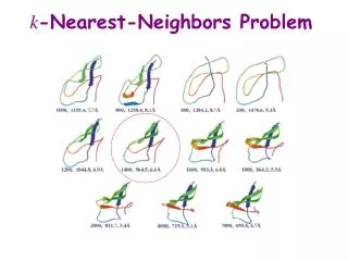
Example: Oil Data Set Figure Bishop 2.28
Implementation Issues • Learning very cheap compared to model estimation. • But prediction expensive: need to retrieve k nearest neighbors from large set of N points, for every prediction. • Nice data structure work: k-d trees, locality-sensitive hashing.
Distance Metric • Does the generalization work. • Needs to be supplied by user. • With Boolean attributes: Hamming distance = number of different bits. • With continuous attributes: Use L2 norm, L1 norm, or Mahalanobis distance. • Also: kernels, see below. • For less sensitivity to choice of units, usually a good idea to normalize to mean 0, standard deviation 1.
Curse of Dimensionality • Low dimension good performance for nearest neighbor. • As dataset grows, the nearest neighbors are near and carry similar labels. • Curse of dimensionality: in high dimensions, almost all points are far away from each other. Figure Bishop 1.21
Point Distribution in High Dimensions • How many points fall within the 1% outer edge of a unit hypercube? • In one dimension, 2% (x < 1%, x> 99%). • In 200 dimensions? Guess... • Answer: 94%. Similar question: to find 10 nearest neighbors, what is the length of the average neighbourhoodcube?
Local Regression • Basic Idea: To predict a target value y for data point x, apply interpolation/regression to the neighborhood of x. • Simplest version: connect the dots.
k-nearest neighbor regression • Connect the dots uses k = 2, fits a line. • Ideas for k =5. • Fit a line using linear regression. • Predict the average target value of the k points.
Local Regression With Kernels • Spikes in regression prediction come from in-or-out nature of neighborhood. • Instead, weight examples as function of the distance. • A homogenous kernel function maps the distance between two vectors to a number, usually in a nonlinear way.k(x,x’) = k(distance(x,x’)). • Example: The quadratic kernel.
The Quadratic Kernel • k = 5 • Let query point be x = 0. • Plot k(0,x’) = k(|x’|).
Kernel Regression • For each query point xq, prediction is made as weighted linear sum: y(xq) = wxq. • To find weights, solve the following regression on the k-nearest neighbors: