Electro-absorption Modulators
Electro-absorption Modulators. EE232, Spring 2001 Pei-Cheng Ku April 24 & 26, 2001. Optical Modulation. Direct modulation on semiconductor lasers: Output frequency drifts carrier induced (chirp) temperature variation due to carrier modulation

Electro-absorption Modulators
E N D
Presentation Transcript
Electro-absorption Modulators EE232, Spring 2001 Pei-Cheng Ku April 24 & 26, 2001
Optical Modulation • Direct modulation on semiconductor lasers: • Output frequency drifts • carrier induced (chirp) • temperature variation due to carrier modulation • Limited modulation depth (don’t want to turn off laser) • External modulation • Electro-optical modulation (low efficiency) • Electroabsorption (EA) modulation (smaller modulation bandwidth)
Electroabsorption (EA) Modulator • EA modulator is a semiconductor device with the same structure as the laser diode. • In laser diodes, we inject large enough current to achieve stimulated emission. While in EA modulator, we apply electric field (reverse bias) to change the absorption spectrum. No carriers are injected into the active region. However, carriers are generated due to absorption of light.
Advantages of EA modulators • Zero biasing voltage • Low driving voltage • Low/negative chirp • high bandwidth • Integrated with DFB
Schematics of an EA modulator • Waveguide type is more popular. From textbook, figure 13.10.
Outline of our discussion • Know how absorption spectrum changes with applied electric field (effective-mass approximation) • See how extinction ratio of modulation can be enhanced in the quantum well (quantum confined Stark effect). Excitons will be introduced. • We will follow the textbook (chapter 13). A recommended reference book is “Introduction to Semiconductor Optics” by N. Peyghambarian et al. (1993).
Physics behind EA Modulators • How absorption spectrum in semiconductors can be changed? • Physical model: effective-mass equation • Single-particle representation • Two-particel representation • Coulomb interaction between electrons and holes: Excitons • Electric field effect: Franz-Keldysh effect • Coulomb+Electric field: DC Stark effect • Coulomb+Electric field+QW: QCSE
Absorption Spectrum Change under Applied Electric Field • Franz-Keldysh Effect • Neglect Coulomb interaction between electrons and holes. • DC Stark Effect • Franz-Keldysh effect plus Coulomb interaction between electrons and holes (excitons). • Quantum confined Start effect (QCSE) • DC Stark Effect in quantum wells • Excitons been confined in quantum well. Stark effect enhanced.
Effective mass approximation • Electron moving in semiconductor crystal with periodic potential V (r)under the influence of a potential U (r). • Effective mass approximation: if the potential is slowly varying compared to the period of the lattice, the above equation can be replaced by effective-mass equation as follows (section 4.4.1 and appendix B):that is the potential causes the envelope of the fast-varying Bloch function to change. Without potential U (r), the envelope f (r) reduces to plane wave
Wavefunction for electrons moving in periodic potential • For example, at the valence bandedge. The wavefunction is p-like (L = 3/2 in sp3 orbitals).
Form of U (r) • Franz-Keldysh Effect • DC Stark Effect (slow-varying approximation only holds for Wannier excitons) • Quantum confined Start effect (QCSE)
Effective mass approximation in Two-Particle Representation • Since U (r) is in general a function of both electron and hole, it’s more convenient to combine two single-particle equations of motion for electron and hole together. • Effective-mass equation for electrons:Effective-mass equation for holes:Add them together
Effective mass approximation in Two-Particle Representation (cont.) • In the path of generalizing single-particle effective mass equation to two-particle effective mass equation, we didn’t make new approximations. The new envelope wavefunction (which is a linear combination of the single-particle envelope functions for electrons and holes) still has to satisfy the slowly-varying approximation. This will be valid if the potential seen by electrons can be smoothly transferred to the potential profile seen by holes.
Validity of Slowly-Varying Approximationin two-particle representation • Franz-Keldysh EffectFor 5V applied voltage, there is 500kV/cm electric field across 0.1mm active region. The variation of electric field across a lattice site is 500kV/cm x 5.6Å ~ 0.028V which gives an energy variation of 0.028eV for an electron. • For an electron moving in periodic atomic potential, it sees a Coulombic attraction from the nucleus. • The potential energy variation across a lattice site is around V(a) ~ 2.569eV >> 0.028eV!
Excitons • The effective-mass equation for an electron-hole pair is:We have to sum over all possible interactions between electrons and holes. But if the carrier density is low enough, we can neglect the contribution from the rest of the electrons and holes and consider only bare Coulomb interaction, that is:
Effective-mass equation for Excitons • With the bare Coulomb interaction between electron and hole, we have the effective-mass equation for an exciton as follows.This equation is formally identical to a hydrogen atom problem except the masses for the electron and proton are replaced by the effective masses for the electrons and holes, respectively. • Any central-force problem (i.e. the potential is a function of relative coordinate between two particles) can be separated into center-of-mass motion and relative motion.
Center-of-mass motion and Relative motion • Effective-mass equation in two-particle representation for any central-force problem can be rewritten as follows. • Center-of-mass motion is a free-running solution:
Solutions for Excitons • Same as hydrogen atoms (3D or 2D) • Exciton Bohr Radius and Rydberg energyEnergy levels: bound states and continuum • Ionization energy for ground state exciton in 2D case is 4 times larger than it is in 3D case. Therefore in QW, it’s easier to form bound exciton states.
Electron-hole energy E n=3 n=2 n=1 K Energy Diagram of Excitons In GaAs, E1=4.2meV (3D) or E1=16.8meV (2D) continuum
Wavefunction for Excitons (3D) • Coulomb potential is spherical symmetric with respect to the center of mass. • Three quantum numbers: n, l, m. • “Accidental degeneracy” for same quantum number n. Orbitals designated by 1s, 2s, 2p, 3s, 3p, 3d, …
probability 1s 2s 2p r/aB Radial Solution (3D)
s-like electron (L=1/2) bloch function P-like exciton envelope function (e.g. n=2) S-like exciton envelope function (e.g. n=1) p-like hole (L=3/2) bloch function Wavefunction Representation for Excitons (3D) Sitting at hole reference frame.
Wavefunction for Excitons (2D) • Coulomb potential is cylindrical symmetric with respect to the center of mass. • Two quantum numbers: n, m. • “Accidental degeneracy” for same quantum number n.
Radial Solution (2D) 2D excitons are more tightly bounded.
Validity of Approximations used in the Calculation of Excitons • Slowly-Varying Potential Profile Approximation:GaAs/InGaAs/AlGaAs lattice density ~ 5.6Å • Bare Coulomb interaction approximation:Exciton radius aB for GaAs ~ 140ÅExciton density: 3D: 8.7e16/cm-3 2D: 8.1e10/cm-2 • For EA modulators, no carriers are injected into active region. Carrier density ~ intrinsic doping level ~ 1e16/cm-3 (bulk) or 1e10/cm-2 (100Å QW). Bare coulomb interaction is a good approximation. • But for laser applications, carrier density is high: 5e18/cm-3 (bulk) or 5e12/cm-2 (100Å QW). Coulomb interaction between electrons and holes is screened.
Optical Absorption without U (r) • From Fermi’s golden rule, the absorption coefficient can be derived as in equation (9.1.23) between two energy bands:where matrix element is calculated as in section 9.3.1 in the case of no external electric field and neglecting the Coulomb interaction between electrons and holes. The result is as follows (equation 9.3.11).
Absorption Spectrum Calculation Summary • Absorption is proportional to the probability that we find electron and hole at the same “position” (i.e. r=0). • For central force problem, we only need to evaluate the envelope wavefunction for the relative motion and take the square of its absolute value. • Note the factor of 2 in the formula of the absorption spectrum comes from the fact that we consider two particles at one time. • The delta function takes care of the (joint) density of states available. • We have to sum over all possible states to get the total absorption.
Remarks on the first assertion • Same “position” actually means electron and hole are in the same lattice site. What happens in the unit cell is governed by the oscillation strength pcv which depends on the details of the Bloch functions inside the lattice site. • This is because is an “envelope” function. The true wavefunction is the product of the envelope function with the Bloch function. • is the probability of finding the electron and hole in the same lattice site.
Density of States function g (E) • Density of states means total number of degenerate states for a given energy level. For example in bulk materials, since there’s no restriction on the motion of the electrons, for a given energy E, the number of states that satisfyis the density of states at that energy.
0D 1D g(E) 3D 2D E Diagrammatic representation for g (E) For a given energy range, the number of carriers necessary to fill out these density of states: 3D>2D>1D>0D.
Franz-Keldysh Effect • Franz-Keldysh effect is also a central-force problem.
Ai(Z) Z Airy Function Ai (Z) • Z>0: electron-hole energy+Eg < electric field potential • Z<0: electron-hole energy+Eg > electric field potential, i.e. above bandgap oscillation wavefunction Smaller period
Absorption Spectrum of Franz-Keldysh Effect • Absorption spectrum reduce to the familiar square root dependence of energy when F0.
Exciton Absorption Spectrum • 3D Excitons • 2D Excitons
Exciton Absorption Spectra (schematics) • 2D and 3D exciton absorption spectra with zero/finite linewidth. The spectra is very sensitive to the temperature. With damping Without damping
Excitonic effect at different temperature T Bulk GaAs Absorption peak blueshifts because the bandgap becomes larger at lower temperature. Quantum well (quasi 2D)
Sommerfeld Enhancement • Even without excitonic peaks, bandedge absorption is enhanced due to Coulombic interaction between electrons and holes. Lots of bound states near the onset of continnum sum together to give Sommerfeld enhancement.
Quantum Confined Stark Effect* • Because the potential of the quantum well breaks the spherical symmetry, it’s not a central force problem anymore! This symmetry breaking, unfortunately, forces us to solve this problem numerically. However, we’ll try to factorize this equation and get more physical insights. Quantum well potential *D. A. B. Miller et al., Phys. Rev. B., 32, 1043 (1985)
Solutions to QCSE • Consider solutions inside the quantum well. For given z, we can see that the problem reduces to 2D-exciton problem. For given r, this is a quantum well problem. Therefore we can expect the solution to this equation can be expanded in terms of the product of 2D-exciton envelope function and the quantum well wavefunction. We then expect that this expansion should only need a few terms to give a good approximation. • Physically, because of the carrier confinement due to the quantum well, we should expect most of the excitons have their electron and hole either both in the quantum well or both outside the quantum well. • As we have seen before, 2D exciton has 4 times larger ionization energy and therefore is much more stable than excitons outside the quantum well.
Absorption Spectrum for QCSE • Exciton absorption peak red-shifts with increasing electric field strength.
Absorption peak shifts quadratically with applied electric field • If the quantum well “only perturbs” the solution a little bit, the absorption peak position shift can be calculated from time-independent perturbation theory. • The energy shift, for example for the ground state exciton in infinite quantum well, due to the electric field is:Absorption peak shifts quadratically with applied electric field. Potential profile has reflection symmetry along z-direction. Thus exciton wavefunction is either even or odd with respect to z=0.
Design considerations for EA modulators • Operation principle • Contrast ratio • Insertion loss • Modulation efficiency • Chirp considerations and optimization • Packaging and Integration
EA Modulators use QCSE • By applying electric field parallel to the quantum well growth direction, the absorption can be changed dramatically at the desired wavelength.
Contrast Ratio • The larger the contrast ratio, the better it is. • Contrast ratio can be made as large as possible by increasing the length of the modulator. But propagation loss then becomes an issue.
Insertion Loss • The longer the modulator is, the larger the insertion loss. Therefore, contrast ratio should not be increased by lengthen the device too much. • Waveguide structure also needs careful design to increase the coupling efficiency from the single-mode-fiber output.
Modulation Efficiency • Modulation efficiency quantifies how much voltage do we need to modulate the optical signal. • Smaller detuning will increase the modulation efficiency. However, it also results in a larger insertion loss.