Download
1 / 29
290 likes | 350 Vues
Learn notation, domain, graphs, and level curves for multi-variable functions in mathematics. Understand operations and domains for functions of several variables through examples and illustrations.

E N D
Chapter 8: Functions of Several Variables Section 8.1 Introduction to Functions of Several Variables Written by Karen Overman Instructor of Mathematics Tidewater Community College, Virginia Beach Campus Virginia Beach, VA With Assistance from a VCCS LearningWare Grant
In this lesson we will discuss: • Notation of functions of several variables • Domain of functions of several variables • Graphs of functions of several variables • Level curves for functions of several variables
Notation for Functions of Several Variables Previously we have studied functions of one variable, y = f(x) in which x was the independent variable and y was the dependent variable. We are going to expand the idea of functions to include functions with more than one independent variable. For example, consider the functions below:
Hopefully you can see the notation for functions of several variables is similar to the notation you’ve used with single variable functions. The function z = f(x, y) is a function of two variables. It has independent variables x and y, and the dependent variable z. Likewise, the function w = g(x, y, z) is a function of three variables. The variables x, y and z are independent variables and w is the dependent variable. The function h is similar except there are four independent variables.
When finding values of the several variable functions instead of just substituting in an x-value, we will substitute in values for each of the independent variables: For example, using the function f on the previous slide, we will evaluate the function f(x, y) for (2, 3) , (4, -3) and (5, y).
A Function of Two Variables: A function f of two variables x and y is a rule that assigns to each ordered pair (x, y) in a given set D, called the domain, a unique value of f. Functions of more variables can be defined similarly. The operations we performed with one-variable functions can also be performed with functions of several variables. For example, for the two-variable functions f and g: In general we will not consider the composition of two multi-variable functions.
Domains of Functions of Several Variables: Unless the domain is given, assume the domain is the set of all points for which the equation is defined. For example, consider the functions The domain of f(x,y) is the entire xy-plane. Every ordered pair in the xy-plane will produce a real value for f. The domain of g(x, y) is the set of all points (x, y) in the xy-plane such that the product xy is greater than 0. This would be all the points in the first quadrant and the third quadrant.
Example 1: Find the domain of the function: Solution: The domain of f(x, y) is the set of all points that satisfy the inequality: or You may recognize that this is similar to the equation of a circle and the inequality implies that any ordered pair on the circle or inside the circle is in the domain. y The highlighted area is the domain to f. x
Example 2: Find the domain of the function: Solution: Note that g is a function of three variables, so the domain is NOT an area in the xy-plane. The domain of g is a solid in the 3-dimensional coordinate system. The expression under the radical must be nonnegative, resulting in the inequality: This implies that any ordered triple outside of the sphere centered at the origin with radius 4 is in the domain.
Example 3: Find the domain of the function: Solution: We know the argument of the natural log must be greater than zero. So, This occurs in quadrant I and quadrant III. The domain is highlighted below. Note the x-axis and the y-axis are NOT in the domain. y x
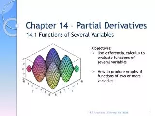
Graphs of Functions of Several Variables As you learned in 2-dimensional space the graph of a function can be helpful to your understanding of the function. The graph gives an illustration or visual representation of all the solutions to the equation. We also want to use this tool with functions of two variables. The graph of a function of two variables, z = f(x, y), is the set of ordered triples, (x, y, z) for which the ordered pair, (x, y) is in the domain. *The graph of z = f(x, y) is a surface in 3-dimensional space. The graph of a function of three variables, w = f(x, y, z) is the set of all points (x, y, z, w) for which the ordered triple, (x, y, z) is in the domain. *The graph of w = f(x, y, z) is in 4 dimensions. We can’t draw this graph or the graphs of any functions with 3 or more independent variables.
Example 4: Find the domain and range of the function and then sketch the graph. Solution: From Example 1 we know the domain is all ordered pairs (x, y) on or inside the circle centered at the origin with radius 5. All ordered pairs satisfying the inequality: The range is going to consist of all possible outcomes for z. The range must be nonnegative since z equals a principle square root and furthermore, with the domain restriction: , the value of the radicand will only vary between 0 and 25. Thus, the range is .
Solution to Example 4 Continued: Now let’s consider the sketch of the function: Squaring both sides and simplifying: You may recognize this equation from Chapter 7 - A sphere with radius 5. This is helpful to sketching the function, but we must be careful !! The function and the equation are not exactly the same. The equation does NOT represent z as a function of x and y – meaning there is not a unique value for z for each (x, y). Keep in mind that the function had a range of , which means the function is only the top half of the sphere.
As you have done before when sketching a surface in 3-dimensions it may be helpful for you to use the traces in each coordinate plane. 1. The trace in the xy-plane, z = 0, is the equation: The circle centered at the origin with radius 5 in the xy-plane. 2. The trace in the yz-plane, x = 0, is the equation: The circle centered at the origin with radius 5 in the yz-plane. 3. The trace in the xz-plane, y = 0, is the equation: The circle centered at the origin with radius 5 in the xz-plane.
Along with sketching the traces in each coordinate plane, it may be helpful to sketch traces in planes parallel to the coordinate planes. 4. Let z = 3: So on the plane z = 3, parallel to the xy-plane, the trace is a circle centered at (0,0,3) with radius 4. 5. Let z = 4: So on the plane z = 4, parallel to the xy-plane, the trace is a circle centered at (0,0,4) with radius 3.
Here is a SKETCH with the three traces in the coordinate planes and the additional two traces in planes parallel to the xy-plane. Keep in mind that this is just a sketch. It is giving you a rough idea of what the function looks like. It may also be helpful to use a 3-dimensional graphing utility to get a better picture. z = 4 z = 3
Here is a graph of the function using the 3-dimensional graphing utility DPGraph. z y x
Example 5: Sketch the surface: Solution: The domain is the entire xy-plane and the range is . 1. The trace in the xy-plane, z = 0, is the equation: Circle 2. The trace in the yz-plane, x = 0, is the equation: Parabola 3. The trace in the xz-plane, y = 0, is the equation: Parabola
Solution to Example 5 Continued: Traces parallel to the xy-plane include the following two. 4. The trace in the plane, z = 5, is the equation: Circle centered at (0, 0, 5) with radius 2. 5. The trace in the plane, z = -7, is the equation: Circle centered at (0, 0, -7) with radius 4.
Here is a sketch of the traces in each coordinate plane. This paraboloid extends below the xy-plane. z y x
Level Curves In the previous two examples, traces in the coordinate planes and traces parallel to the xy-plane were used to sketch the function of two variables as a surface in the 3-dimensional coordinate system. When the traces parallel to the xy-plane or in other words, the traces found when z or f(x,y) is set equal to a constant, are drawn in the xy-plane, the traces are called level curves. When several level curves, also called contour lines, are drawn together in the xy-plane the image is called a contour map.
Example 6: Sketch a contour map of the function in Example 4, using the level curves at c = 5,4,3,2,1 and 0. Solution: c = a means the curve when z has a value of a.
Solution to Example 6 Continued: Contour map with point (0, 0) for c = 5 and then circles expanding out from the center for the remaining values of c. Note: The values of c were uniformly spaced, but the level curves are not. When the level curves are spaced far apart (in the center), there is a gradual change in the function values. When the level curves are close together (near c = 5), there is a steep change in the function values.
Example 7: Sketch a contour map of the function, using the level curves at c = 0, 2, 4, 6 and 8. Solution: Set the function equal to each constant.
Solution to Example 7 Continued: Contour map with point (0, 0) for c = 0 and then ellipses expanding out from the center for the remaining values of c.
Example 7 Continued: Here is a graph of the surface .
Note: • Sketching functions of two variables in 3-dimensions is challenging and will take quite a bit of practice. Using the traces and level curves can be extremely beneficial. • In the beginning, using 3-dimensional graphing utility will help you visualize the surfaces and see how the traces and level curves relate. • 2. The idea of a level curve can be extended to functions of three variables. If w = g(x, y, z) is a function of three variables and k is a constant, then g(x, y, z) = k is considered a level surface of the function g. Though we may be able to draw the level surface, we still cannot draw the function g in 4 dimensions.
Practice problems for this lesson are available in Blackboard under Chapter 8, 8.1 A and B.