Linear Programming
Linear Programming. Overview Formulation of the problem and example I ncremental, deterministic algorithm Randomized algorithm Unbounded linear programs Linear programming in higher dimensions.

Linear Programming
E N D
Presentation Transcript
Linear Programming • Overview • Formulation of the problem and example • Incremental, deterministic algorithm • Randomized algorithm • Unbounded linear programs • Linear programming in higher dimensions Computational Geometry Prof. Dr. Th. Ottmann
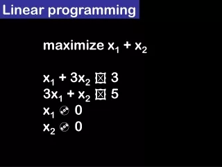
Linear program of dimension d: c = (c1,c2,...,cd) hi = {(x1,...,xd) ; ai,1x1 + ... + ai,dxd bi} Problem description Maximize c1x1 + c2x2 + ... + cdxd Subject to the conditions: a1,1x1 + ... a1,dxd b1 a2,1x1 + ... a2,dxd b2 : : : an,1x1 + ... an,dxd bn li = hyperplane that bounds hi (straight lines, ifd=2) H = {h1, ... , hn} Computational Geometry Prof. Dr. Th. Ottmann
C C C Structure of the feasible region 1. Bounded 2. Unbounded 3. Empty Computational Geometry Prof. Dr. Th. Ottmann
Bounded linear programs • Assumption : • Algorithm UnboundedLP(H, c) yields either • a ray in∩H, which is unbounded towards c, or • two half planes h1 and h2, so that h1 h2 is bounded towards c, or • the answer, that LP(H, c) has no solution, because the feasible region is empty. Computational Geometry Prof. Dr. Th. Ottmann
Incremental algorithm Let C2 = h1 h2 Remaininghalfplanes: h3,..., hn Ci = Ci-1 hi = h1 ... hi Compute-optimal-vertex (H, c) v2 := l1 l2 ; C2 := h1 h2 for i := 3 to n do Ci := Ci-1 hi vi := optimal vertex of Ci C2C3 C4 ... Cn = C Ci = C = Computational Geometry Prof. Dr. Th. Ottmann
Optimal Vertex Lemma 1:Let2 < i n, then we have : 1.If vi-1 hi, then vi = vi-1. 2.If vi-1 hi, then either Ci = or vi li, where li is the line bounding hi. Computational Geometry Prof. Dr. Th. Ottmann
h4 h1 h3 v3= v4 h2 h4 h1 h3 c h5 c h2 v4 v5 Optimal vertex Computational Geometry Prof. Dr. Th. Ottmann
Next optimal vertex fc(x) = c1x1 + c2x2 Ci-1 vi-1 Computational Geometry Prof. Dr. Th. Ottmann
Algorithm 2D-LP Input: A 2-dimensional Linear Program (H, c ) Output: Either one optimal vertex or or a ray along which (H, c ) is unbounded. if UnboundedLP(H, c ) reports (H, c ) is unbounded or infeasible thenreturn UnboundedLP(H, c ) else report h1 := h; h2 := h´ ; v2 := l1 l2 let h3,...,hn be the remaining half-planes of H for i:= 3 to n do if vi-1 hi then vi := vi-1 else Si-1 := Hi-1 * li vi := 1-dim-LP(Si-1, c ) if vi not exists then return return vn Running time: O(n²) Computational Geometry Prof. Dr. Th. Ottmann
Algorithm 1D-LP Computational Geometry Prof. Dr. Th. Ottmann
Algorithm 1D-LP • Find the point x on li that maximizes cx , subject to • the constraints x hj, for 1 j i –1 • Observation: li hj is a ray • Let si-1 := { h1 li, ..., hi-1 li} • Algorithm 1D-LP{si-1, c } • p1 = s1 • for j := 2 to i-1 do pj = pj-1 sj • if pi-1then • return the optimal vertex of pi-1else • return • Time: O(i) Computational Geometry Prof. Dr. Th. Ottmann
Bad 11 12 9 10 7 8 5 6 3 4 1 2 vi Good 1 2 3 4 5 6 7 8 9 10 11 12 Addition of halfplanes in different orders Computational Geometry Prof. Dr. Th. Ottmann
h4 h1 h3 v3= v4 h2 h4 h1 h3 c h5 c h2 v4 v5 Optimal vertex Computational Geometry Prof. Dr. Th. Ottmann
Algorithm 2D-LP Input: A 2-dimensional Linear Program (H, c ) Output: Either one optimal vertex or or a ray along which (H, c ) is unbounded. if UnboundedLP(H, c ) reports (H, c ) is unbounded or infeasible thenreturn UnboundedLP(H, c ) else report h1 := h; h2 := h´ ; v2 := l1 l2 let h3,...,hn be the remaining half-planes of H for i:= 3 to n do if vi-1 hi then vi:=vi-1 else Si-1:= Hi-1 * li vi:= 1-dim-LP(Si-1, c ) if vi not exists then return return vn Running time: O(n²) Computational Geometry Prof. Dr. Th. Ottmann
Bad 11 12 9 10 7 8 5 6 3 4 1 2 vi Good 1 2 3 4 5 6 7 8 9 10 11 12 Addition of halfplanes in different orders Computational Geometry Prof. Dr. Th. Ottmann

