Column Buckling - Inelastic
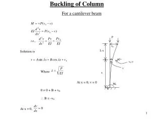
Column Buckling - Inelastic. A long topic. Effects of geometric imperfection. v o. v. Leads to bifurcation buckling of perfect doubly-symmetric columns. P. M x. v. P. Effects of Geometric Imperfection. Geometric Imperfection. A F = amplification factor. Geometric Imperfection.


Column Buckling - Inelastic
E N D
Presentation Transcript
Column Buckling - Inelastic A long topic
Effects of geometric imperfection vo v Leads to bifurcation buckling of perfect doubly-symmetric columns P Mx v P
Geometric Imperfection AF = amplification factor
Geometric Imperfection Increases exponentially Limit AF for design Limit P/PE for design Value used in the code is 0.877 This will give AF = 8.13 Have to live with it.
History of column inelastic buckling • Euler developed column elastic buckling equations (buried in the million other things he did). • Take a look at: http://en.wikipedia.org/wiki/EuleR • An amazing mathematician • In the 1750s, I could not find the exact year. • The elastica problem of column buckling indicates elastic buckling occurs with no increase in load. • dP/dv=0
History of Column Inelastic Buckling • Engesser extended the elastic column buckling theory in 1889. • He assumed that inelastic buckling occurs with no increase in load, and the relation between stress and strain is defined by tangent modulus Et • Engesser’s tangent modulus theory is easy to apply. It compares reasonably with experimental results. • PT=ETI / (KL)2
History of Column Inelastic Buckling • In 1895, Jasinsky pointed out the problem with Engesser’s theory. • If dP/dv=0, then the 2nd order moment (Pv) will produce incremental strains that will vary linearly and have a zero value at the centroid (neutral axis). • The linear strain variation will have compressive and tensile values. The tangent modulus for the incremental compressive strain is equal to Et and that for the tensile strain is E.
History of Column Inelastic Buckling • In 1898, Engesser corrected his original theory by accounting for the different tangent modulus of the tensile increment. • This is known as the reduced modulus or double modulus • The assumptions are the same as before. That is, there is no increase in load as buckling occurs. • The corrected theory is shown in the following slide
History of Column Inelastic Buckling • The buckling load PR produces critical stress R=Pr/A • During buckling, a small curvature d is introduced • The strain distribution is shown. • The loaded side has dL and dL • The unloaded side has dU and dU
History of Column Inelastic Buckling • S1 and S2 are the statical moments of the areas to the left and right of the neutral axis. • Note that the neutral axis does not coincide with the centroid any more. • The location of the neutral axis is calculated using the equation derived ES1 - EtS2 = 0
History of Column Inelastic Buckling E is the reduced or double modulus PR is the reduced modulus buckling load
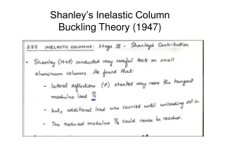
History of Column Inelastic Buckling • For 50 years, engineers were faced with the dilemma that the reduced modulus theory is correct, but the experimental data was closer to the tangent modulus theory. How to resolve? • Shanley eventually resolved this dilemma in 1947. He conducted very careful experiments on small aluminum columns. • He found that lateral deflection started very near the theoretical tangent modulus load and the load capacity increased with increasing lateral deflections. • The column axial load capacity never reached the calculated reduced or double modulus load. • Shanley developed a column model to explain the observed phenomenon
Column Inelastic Buckling P dP/dv=0 Slope is zero at buckling P=0 with increasing v v Elastic buckling analysis • Three different theories • Tangent modulus • Reduced modulus • Shanley model • Tangent modulus theory assumes • Perfectly straight column • Ends are pinned • Small deformations • No strain reversal during buckling PT
Tangent modulus theory v Mx PT • Assumes that the column buckles at the tangent modulus load such that there is an increase in P (axial force) and M (moment). • The axial strain increases everywhere and there is no strain reversal. Strain and stress state just before buckling PT T T=PT/A Strain and stress state just after buckling Mx - Pv = 0 T T v T=ETT T Curvature = = slope of strain diagram
Tangent modulus theory • Deriving the equation of equilibrium • The equation Mx- PTv=0 becomes -ETIxv” - PTv=0 • Solution is PT= 2ETIx/L2
Example - Aluminum columns • Consider an aluminum column with Ramberg-Osgood stress-strain curve
Residual Stress Effects b x d y • Consider a rectangular section with a simple residual stress distribution • Assume that the steel material has elastic-plastic stress-strain curve. • Assume simply supported end conditions • Assume triangular distribution for residual stresses rc rc rt y y y/b y y E
Residual Stress Effects • One major constrain on residual stresses is that they must be such that • Residual stresses are produced by uneven cooling but no load is present
Residual Stress Effects b • Response will be such that - elastic behavior when x d y b b x y Y Y Y/b
b b x y
b b x y
Tangent modulus buckling - Numerical Afib yfib Centroidal axis Discretize the cross-section into fibers Think about the discretization. Do you need the flange To be discretized along the length and width? 1 For each fiber, save the area of fiber (Afib), the distances from the centroid yfib and xfib, Ix-fib and Iy-fib the fiber number in the matrix. 2 Discretize residual stress distribution 3 Calculate residual stress (r-fib) each fiber 4 Check that sum(r-fib Afib)for Section = zero 5
Tangent Modulus Buckling - Numerical Calculate the critical (KL)X and (KL)Y for the (KL)X-cr = sqrt [(EI)Tx/P] (KL)y-cr = sqrt [(EI)Ty/P] 14 Calculate effective residual strain (r) for each fiber r=r/E 6 Calculate the tangent (EI)TX and (EI)TY for the (EI)TX = sum(ET-fib{yfib2 Afib+Ix-fib}) (EI)Ty = sum(ET-fib{xfib2 Afib+ Iy-fib}) 13 Assume centroidal strain 7 Calculate average stress = = P/A 12 Calculate total strain for each fiber tot=+r 8 Calculate Axial Force = P Sum (fibAfib) 11 Assume a material stress-strain curve for each fiber Calculate stress in each fiber fib 10 9