Download
1 / 37
380 likes | 562 Vues
Inferring Solar Internal Structure and Rotation from p-mode Frequencies and Splittings I. Michael Thompson University of Sheffield, UK Affiliate scientist, High Altitude Observatory. Commercial break. Postdoctoral Research Associate

E N D
Inferring Solar Internal Structure and Rotation from p-mode Frequencies and Splittings I Michael Thompson University of Sheffield, UK Affiliate scientist, High Altitude Observatory
Commercial break Postdoctoral Research Associate Department of Applied Mathematics, University of Sheffield, UK The post holder will be required to undertake research in local helioseismology. The post holder must have a PhD in applied mathematics, solar physics, astrophysics or similar area and will have demonstrated the ability to write numerical code to solve coupled boundary value partial differential equations. The ability to carry out calculations (e.g. Green’s functions, Fourier transforms etc.) and familiarity with MHD, scattering processes and helioseismology is also desirable. This post is available from 1 October 2005 (or soon thereafter) for a period of up to 30 months. Enquiries to Dr. Rekha Jain R.Jain@sheffield.ac.uk Full details/application packs: www.shef.ac.uk/jobs/jobs_all.html Email: Jobs@Sheffield.ac.uk Reference PR2202 Closing Date: 05/09/2005
Helioseismic inversion Forward modeling Model Observables Inversion Aim of inversion: to make inferences about (usually) localized properties of the solar interior
Vertical wavenumber Standing-wave condition, with surface phase shift a Inferring solar sound speed as a function of depth Recall from JCD lecture on asymptotic mode properties: Hence Duvall law i.e. F(w) = (n+α)π/ω , where w = ω/L. Can determine RHS observationally and hence find F(w). We can then use F(w) to determine sound speed c(r).
Observed Duvall law F(w)
Abel inversion Have measured F(w); want to find c(r).
w a as Change order of integration: as a a Do w integral with a change of variable:
Hence, finally This gives r as a function of a and hence implicitly a=c/r as a function of r and hence c as a function of r.
0.3 0.2 c2 (Mm s-1)2 0.1 0 0 0.2 0.4 0.6 0.8 1.0 r / R First inversion of solar data Convection-zone base Solid curve: inversion of solar data Dashed curve: solar model From Christensen-Dalsgaard et al. (1985) Nature 315, 378
Linear inversion methods Many of the inversion methods used in helioseismology are linear: the solution is a linear function of the data. In the rest of this lecture I shall introduce some linear techniques and a framework for understanding and comparing them, in the context of a simple application. In the next lecture we shall apply these techniques to studying the Sun’s 2-D rotation profile and its internal structure.
Prototypical example:1-D rotation law Ω(r) As discussed by JCD, rotation raises the degeneracy of global mode frequencies and introduces a dependence on azimuthal order m. The dependence is particularly simple if we consider a rotation profile Ω(r) depending only on the radial coordinate: The kernels Knl(r) are different for different modes.
Kernels Knl(r) for 1-D rotation Low-degree mode Medium-degree mode
Let dnl = (ωnlm- ωnl0)/m be our data. Then where εnl are noise in the data, each with with standard deviation (s.d.) σnl. For simplicity, we shall use single subscript “i” in place of “nl”.
Least-squares fitting Idea of least-squares (LS) fitting: Approximate the unknown function Ω(r) in terms of a chosen set of basis functions φk(r): Ω(r)≈ Ω(r) = Σxkφk(r) . Choose coefficients xk to minimize
This can be written as a matrix equation: minimize | Ax – b |2 . The solution of this is x = ( ATA)-1AT b . Unfortunately, unless we choose a highly restrictive representation for Ω, the matrix A is usually ill-conditioned in helioseismic inversions and so the LS solution x and hence Ω also are dominated by data noise and thus useless.
Regularized Least-Squares (RLS) fitting We can get better-behaved solutions out of LS by adding a “regularization term” to the minimization: e.g. to minimize trade-off parameter or This can again be written as a matrix equation: minimize | Ax – b |2 + λ2| Lx |2 . The solution is x = ( ATA + λ2 LTL)-1AT b .
Optimally Localized Averages (OLA) method Idea: for each radial location r0, try to find a linear combination of the kernels that is localized there. If successful, then the same linear combination of the data is a localized average of the rotation rate near r=r0:
How can the coefficients ci be found? OLA Classic (Multiplicative OLA – MOLA) Choose the coefficients ci so as to minimize E.g. J=12(r-r0)2. This penalizes K for being large except at r=r0. Parameter θ trades off between localizing K and keeping the error term small Subtractive OLA (SOLA) Choose the coefficients ci so as to minimize E.g. T=A exp(-(r-r0)2/ δ2). This penalizes K for deviating from the target function T. Trade-off parameters: θ and δ.
Error propagation Assume the errors in the individual data di are independent (i.e. uncorrelated) and the standard deviation of each di is σi, say. If the solution is Ω(r0) = Σ ci di then the standard deviation σ[Ω(r0)] in the solution is is given by σ[Ω(r0)] = (Σ ci2di2 )1/2
Error correlation Consider the solution at two points r1 and r2: Ω(r1) = Σ c1i di , Ω(r2) = Σ c2i di These are constructed from the same (noisy) data and so in general their errors are correlated, i.e. cov[Ω(r1) , Ω(r2) ] = E[(Ω(r1) –E[Ω(r1)]) (Ω(r2) –E[Ω(r2)])] ≠ 0 If the data errors are independent: cov[Ω(r1) , Ω(r2)] = Σ c1i c2i σi2
A common framework for discussing any linear inversion LS, RLS, MOLA, SOLA techniques above are all examples of linear methods: the solution is a linear combination of the data. For any linear method, we can find inversion coefficients ci(r0), look at averaging kernels Σci(r0)Ki(r) and calculate error propagation, using the same expressions as in OLA.
Examples of averaging kernels OLA Averaging kernels for Ω(r) constructed with 834 p-modes with 1 ≤ l≤ 200 Note that the RLS kernels have negative sidelobes and near- surface structure. RLS
Inversion coefficients Inversion coefficients for solution at r0=0.5R, for OLA and RLS inversions and (continuous curve) for a linear asymptotic inversion method. OLA RLS
Trade-off curves L-curve Global measures for RLS method At a point – for any linear method | Lx | Size of error bar Averaging kernel width | Ax – b |
RLS OLA
SVD analysis to understand what’s happening in (R)LS Can make singular value decomposition (SVD) of matrix A : A = U Σ VT where U and V are orthogonal matrices (i.e. UTU=I and VTV=I) with column vectors u(i) and v(i) say, and Σ = diag(s1,s2,…,sR) is a diagonal matrix whose elements are the singular values of s1 ≥ s2 ≥ … ≥ sR of matrix A
Least-squares solution: x = (ATA)-1ATb = V Σ-1UTb. Hence Small singular values cause any errors in b to “blow up” in the solution. This is why unregularized least-squares hits a problem. Note the roles of U and V: the data are projected onto the u(i), while the v(i) form a basis for the solution vector x.
Truncated SVD inversion Since small singular values cause a problem, one egularization method is just to truncate the summation at j=K, say, when the singular values go below some threshold value:
It turns out that the solution of the RLS problem with regularization in standard form is This is like the unregularized solution but each term is multiplied by a “filter” fi = si2 / (λ2+si2). When si » λ, fi ≈ 1; when si« λ, fi ≈ 0. This is like truncated SVD but with a smoother cut-off.
This can be generalized to the RLS solution with a general smoothing matrix L. One needs the generalized singular value decomposition (GSVD) of the matrix pair (A,L): A = U diag(αi) W-1 , L = V diag(βi) W-1 ; Then where (roughly) fi = γi2/(λ2+ γi2) with γi = αi / βi . See Christensen-Dalsgaard et al. (1993), MNRAS 264, 541 for the details.
Further reading: Gough, D. (1985). Inverting helioseismic data. Solar Physics 100, 65-99. Christensen-Dalsgaard, J. et al. (1990). A comparison of methods for inverting helioseismic data. Mon. Not. R. astr. Soc. 242, 353-369.
Observed Duvall law F(w)