Multivariate Genetic Analysis
Learn about Cholesky decomposition and genetic analysis using MRI and IQ data to partition genetic, shared, and specific environmental factors. Explore the independent pathway model with an example script.

Multivariate Genetic Analysis
E N D
Presentation Transcript
Multivariate Genetic Analysis Boulder 2004
1.00 1.00 1.00 1.00 F1 F2 F3 F4 P1 P2 P3 P4 T1 T1 T1 T1 Phenotypic Cholesky
1.00 1.00 1.00 1.00 F1 F2 F3 F4 P1 P2 P3 P4 T1 T1 T1 T1 Phenotypic Cholesky
1.00 1.00 1.00 1.00 F1 F2 F3 F4 P1 P2 P3 P4 T1 T1 T1 T1 Phenotypic Cholesky
1.00 1.00 1.00 1.00 F1 F2 F3 F4 P1 P2 P3 P4 T1 T1 T1 T1 Phenotypic Cholesky
Cholesky Example • Script: f:\hmaes\a17\chol.mx • 3 MRI measures – 2 IQ subtests: • var1 = cerebellum • var2 = grey matter • var3 = white matter • var4 = calculation • var5 = letters and numbers • Data: f:\hmaes\a17\mri-iqfactor.rec • T:\hmaes/a17\mri-iq-mz.dat • T:\hmaes\a17\mri-iq-dz.dat
Cholesky #define nvar 5 Begin Matrices; X lower nvar nvar Free ! genetic structure Y lower nvar nvar Free ! shared environment structure Z lower nvar nvar Free ! specific environment structure M full 1 nvar Free ! grand means End Matrices; Begin Algebra; A= X*X'; ! additive genetic covariance C= Y*Y'; ! shared environment covariance E= Z*Z'; ! nonshared environment covariance End Algebra;
Standardization Begin Algebra; R=A+C+E; ! total variance S=(\sqrt(I.R))~; ! diagonal matrix of standard deviations P=S*X| S*Y| S*Z; ! standardized estimates End Algebra;
1.00 F1 P1 P2 P3 P4 T1 T1 T1 T1 Phenotypic Single Factor
1.00 F1 P1 P2 P3 P4 T1 T1 T1 T1 E1 E2 E3 E4 1.00 1.00 1.00 1.00 Residual Variances
1.00 ? 1.00 F1 F1 P1 P2 P3 P4 P1 P2 P3 P4 T1 T1 T1 T1 T2 T2 T2 T2 E1 E2 E3 E4 E1 E2 E3 E4 1.00 1.00 1.00 1.00 1.00 1.00 1.00 1.00 Twin Data
1.0 / 0.5 1.00 1.00 A1 A1 P1 P2 P3 P4 P1 P2 P3 P4 T1 T1 T1 T1 T2 T2 T2 T2 E1 E2 E3 E4 E1 E2 E3 E4 1.00 1.00 1.00 1.00 1.00 1.00 1.00 1.00 Genetic Single Factor
Single [Common] Factor • X: genetic • Full 4 x 1 • Full nvar x nfac • Y: shared environmental • Z: specific environmental
1.00 1.0 / 0.5 1.00 1.00 1.00 1.00 A1 C1 A1 C1 P1 P2 P3 P4 P1 P2 P3 P4 T1 T1 T1 T1 T2 T2 T2 T2 E1 E2 E3 E4 E1 E2 E3 E4 1.00 1.00 1.00 1.00 1.00 1.00 1.00 1.00 Common Environmental Single Factor
1.00 1.0 / 0.5 1.00 1.00 1.00 1.00 1.00 1.00 A1 C1 E1 A1 C1 E1 P1 P2 P3 P4 P1 P2 P3 P4 T1 T1 T1 T1 T2 T2 T2 T2 E1 E2 E3 E4 E1 E2 E3 E4 1.00 1.00 1.00 1.00 1.00 1.00 1.00 1.00 Specific Environmental Single Factor
1.00 1.0 / 0.5 1.00 1.00 1.00 1.00 1.00 1.00 A1 C1 E1 A1 C1 E1 P1 P2 P3 P4 P1 P2 P3 P4 T1 T1 T1 T1 T2 T2 T2 T2 A1 C1 E1 E2 E3 E4 E1 E2 E3 E4 1.00 1.00 1.00 1.00 1.00 1.00 1.00 1.00 1.00 1.00 Residuals partitioned in ACE
Residual Factors • T: genetic • U: shared environmental • V: specific environmental • Diag 4 x 4 • Diag nvar x nvar
1.00 / 0.50 1.00 1.00 1.00 1.00 1.00 1.00 1.00 A C E A C E C C C C C C [Y] [X] [Z] P1 P2 P3 P4 P1 P2 P3 P4 T1 T1 T1 T1 T2 T2 T2 T2 [V] [U] [T] E1 E2 E3 E4 E1 E2 E3 E4 C1 A1 1.00 A2 1.00 A3 1.00 A4 1.00 A1 1.00 A2 1.00 A3 1.00 A4 1.00 1.00 1.00 1.00 1.00 1.00 1.00 1.00 1.00 1.00 1.00 / 0.50 1.00 / 0.50 1.00 / 0.50 1.00 / 0.50 Independent Pathway Model
Independent Pathway Example • Script: f:\hmaes\a17\ind3f.mx • 3 MRI measures – 2 IQ subtests: • var1 = cerebellum • var2 = grey matter • var3 = white matter • var4 = calculation • var5 = letters and numbers • Data: f:\hmaes\a17\mri-iqfactor.rec • T:\hmaes/a17\mri-iq-mz.dat • T:\hmaes\a17\mri-iq-dz.dat
Independent Pathway #define nvar 5 #define nfac 1 G1: Define matrices Calculation Begin Matrices; X full nvar 3 ! common factor genetic paths Y full nvar nfac ! common factor shared env paths Z full nvar nfac Free ! common factor specific env paths T diag nvar nvar Free ! variable specific genetic paths U diag nvar nvar ! variable specific shared env paths V diag nvar nvar Free ! variable specific residual paths M full 1 nvar Free ! grand means End Matrices;
Three Genetic Factors Specify X ! declare free parameters for 3 genetic common factors ! G1 G2 G3 100 110 0 101 111 0 102 112 0 103 0 120 104 0 121 Drop T 1 5 5 ! fix genetic specific for last variable for identification
1.00 1.00 1.00 A1 A2 A3 CB GM WM RK CL AS1 AS2 AS3 AS4 AS5 1.00 1.00 1.00 1.00 1.00 Three Genetic Factors
Independent II Begin Algebra; A= X*X' + T*T'; ! additive genetic covariance C= Y*Y' + U*U'; ! shared environment covariance E= Z*Z' + V*V'; ! specific environment covariance End Algebra; Begin Algebra; R=A+C+E; ! total variance S=(\sqrt(I.R))~; ! diagonal matrix of standard deviations P=S*X| S*Y| S*Z| \d2v(S*T)'| \d2v(S*U)'| \d2v(S*V)'; ! standardized estimates for common and specific factors End Algebra; \d2v : diagonal to vector
1.00 F1 P1 P2 P3 P4 T1 T1 T1 T1 Phenotypic Single Factor
1.00 1.0 / 0.5 1.00 1.00 1.00 1.00 1.00 1.00 A C E A C E F1 F1 P1 P2 P3 P4 P1 P2 P3 P4 T1 T1 T1 T1 T2 T2 T2 T2 Latent Phenotype
1.00 / 0.50 1.00 1.00 1.00 1.00 1.00 1.00 1.00 A C E A C E C C C C C C [X] [Y] [Z] constraint L L constraint [F] P1 P2 P3 P4 P1 P2 P3 P4 T1 T1 T1 T1 T2 T2 T2 T2 [V] [U] [T] E1 E2 E3 E4 E1 E2 E3 E4 C1 A1 1.00 A2 1.00 A3 1.00 A4 1.00 A1 1.00 A2 1.00 A3 1.00 A4 1.00 1.00 1.00 1.00 1.00 1.00 1.00 1.00 1.00 1.00 1.00 / 0.50 1.00 / 0.50 1.00 / 0.50 1.00 / 0.50 Common Pathway Model
Common Pathway Example • Script: f:\hmaes\a17\comp.mx • 3 MRI measures – 2 IQ subtests: • var1 = cerebellum • var2 = grey matter • var3 = white matter • var4 = calculation • var5 = letters and numbers • Data: f:\hmaes\a17\mri-iqfactor.rec • T:\hmaes/a17\mri-iq-mz.dat • T:\hmaes\a17\mri-iq-dz.dat
Compath Pathway #define nvar 5 #define nfac 1 Begin Matrices; X full nfac nfac Free ! latent factor genetic paths Y full nfac nfac ! latent factor shared env paths Z full nfac nfac Free ! latent factor specific env paths T diag nvar nvar Free ! variable specific genetic paths U diag nvar nvar ! variable specific shared env paths V diag nvar nvar Free ! variable specific residual paths F full nvar nfac Free ! loadings on latent factor M full 1 nvar Free ! grand means End Matrices;
Compath II Begin Algebra; A= F&(X*X') + T*T'; ! genetic variance components C= F&(Y*Y') + U*U'; ! shared environment covariance E= F&(Z*Z') + V*V'; ! specific environment covariance L= X*X' + Y*Y' + Z*Z'; ! variance of latent factor End Algebra; Begin Algebra; R=A+C+E; ! total variance S=(\sqrt(D.R))~; ! diagonal matrix of standard deviations P=S*F| \d2v(S*T)'| \d2v(S*U)'| \d2v(S*V)'; ! standardized estimates for loadings and specific factors W= X*X' | Y*Y'| Z*Z'; ! standardized estimates for latent phenotype End Algebra;
Summary • Independent Pathway Model • Biometric Factors Model • Loadings differ for genetic and environmental common factors • Common Pathway Model • Psychometric Factors Model • Loadings equal for genetic and environmental common factor