1: Introduction

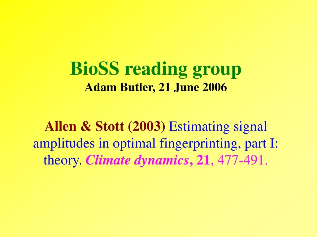
1. BioSS reading groupAdam Butler, 21 June 2006Allen & Stott (2003)Estimating signal amplitudes in optimal fingerprinting, part I: theory.Climate dynamics, 21, 477-491.

2. 1: Introduction • Optimal fingerprinting: statistical methods for climate change detection & attribution • Attempt to assess the extent to which spatial and temporal patterns in observed climate data are related to corresponding patterns within outputs generated by climate models • Assume climate variability independent of externally forced signals of climate change

3. “attribution of observed climate change to a given combination of human activity and natural influences… requires careful assessment of multiple lines of evidence to demonstrate, within a pre-specified margin of error, that the observed changes are: • unlikely to be due entirely to natural variability • consistent with the estimated responses to the given combination of anthropogenic and natural forcing; and • not consistent with alternative explanations of recent climate change that exclude important elements of the given combination of forcings.”

4. The current paper • Optimal fingerprinting is just a particular take on multiple regression • The current paper attempts to deal with one element of climate model uncertainty • Does this by replacing Ordinary Least Squares with Total Least Squares: a standard approach to “errors-in-variables”

5. Model uncertainty • A+S define sampling uncertainty to be - “the variability in the model-simulated response which would be observed if the ensemble of simulations were repeated with an identical model and forcing and different initial conditions…” • They argue this limited definition is difficult to generalise in practice...

6. Avoiding model uncertainty • Restrict attention to mid c21 estimates - signal-to-noise ratio by then so high that inter-ensemble variation is unimportant • Use a purely correlative approach • Use a noise-free model such an energy balance model to simulate response pattern • Use a large number of ensemble runs

7. Problems • Standard optimal fingerprinting uses OLS, estimates can be severely biased towards zero when errors in explanatory variables • Bias particularly problematic when estimating upper limits of uncertainty intervals (Fig. 1)

8. 2.1: Optimal fingerprinting • Basic model: • “Pre-whitening”: find a matrix Psuch that • Rank of P typically [much] smaller than length of y

9. Minimise • P is IID noise, so the solution is: • (ordinary least squares) • Compute confidence intervals based on standard asymptotic distributions…

10. 2.2: Noise variance unknown • Ignoring uncertainty in estimated noise properties can lead to “artificial skill” • Solution: base uncertainty analysis on sets of noise realisations which are statistically independent of those used to estimate P • Obtain such realisations from segments of a control run of a climate model • Elements are not mutually independent…

11. 3. Errors in variables • Extended model: • Pre-whitening: • Seek to solve (Fig. 2)

12. 3.1: Total least squares: estimation of  • Seek to minimise:

13. Solution to the corresponding eigenequation takes s2to be smallest eigenvalue of ZTZ & takes as the corresponding eigenvector • Use a singular value decomposition • Can show that

14. “…in geometric terms minimising s2 is equivalent to finding the m-dimensional plane in an m/-dimensional space which minimises the sum squared perpendicular distance from the plane to the k points defined by the rows of Z…” (Adcock, 1878)

15. 3.2: Total least squares:unknown noise variance • If the same runs are used to derive P and to construct CIs about estimates of  then uncertainty will again be underestimated • As in standard Optimal Fingerprinting, can account for uncertainty in noise variance by using a set of independent control runs…

16. 3.3: Open-ended confidence intervals • The  quantify the ratio of the observed to the model-simulated responses • In TLS we estimate the angle of the slope relating observations to model response • Can obtain highly asymmetric confidence intervals when transform back to  scale via tan(slope) - intervals can even contain infinity

17. 4. Application to a chaotic system • Non-linear system of Palmer & Lorenz, which corresponds to low-order deterministic chaos:

18. Some properties of the Palmer model – • Radically different properties at differ aggregation levels (Figs. 3 & 4) • Sign of response in X direction depends on the amplitude of the forcing (Fig. 5) • Variability at fine resolution changes due to forcing with a plausible amplitude, but variability at coarser resolution does not…

19. A+S choose this system because: • it is a plausible model of true climate - “…Palmer (1999) observed that climate change is a nonlinear system which could also thouht of as a change in the occupancy statistics of certain preferred ‘weather regimes’ in response to external forcing…” • optimal fingerprinting may be expected to have problems with the nonlinearity

20. Use the Palmer model to simulate - • pseudo-observationsy under a linear increase in forcing from 0 to 5 units • spatio-temporal response patternsX for a set of ensemble runs • The level of internal variability using an unforced control run from the model

21. Investigate performance of OLS and TLS, for different numbers of ensembles and different averaging periods (50Ld or 500Ld) • Figure 6: look at the (true) hypothesis =1 • OLS consistently underestimates observed response amplitude for small number of ensembles

22. 5. Discussion • Promoted as an approach to attribution problems when few ensembles are available • Most relevant for low signal-to-noise ratio • Linear: relies on assumption that forcing does not change level of climate variability • Good performance relative to OF with OLS in simulations under deterministic chaos