Understanding SQL Server Query Execution Plans
Learn in-depth about SQL Server query execution plans, covering table and index access methods, join operators, and the importance of understanding execution plans for optimal performance tuning.

Understanding SQL Server Query Execution Plans
E N D
Presentation Transcript
Understanding SQL Server Query Execution Plans Greg Linwood MyDBA gregl@MyDBA.com
About Me • MyDBA • Managed Database Services • SQLskills • SQL Server training • Microsoft SQL Server MVP • Melbourne SQL Server User Group Leader
Agenda • SQL: set based expression / serial execution • Intro to execution plans • Table & index access methods • Table storage formats – Heaps & Clustered Indexes • Nonclustered Indexes (on Heaps vs on Clustered Indexes) • Covering Indexes • Join operators • Nested Loops Join, Merge Join & Hash Join • Review • Discussion
Intro to execution plans • Why is understanding Execution Plans important? • Provides insight into query execution steps / processing efficiency • - SQL Server occasionally makes mistakes • Tune performance problems at the source (query efficiency) • More effective than tuning hardware • Other diagnostics only reveal consequences of poor query execution plans • High CPU is only a consequence of poorly tuned query plans • High disk utilisation usually just a consequence of poorly tuned query plans • Waitstats reveals high resource utilisation of poorly tuned query plans • Locking usually just a consequence of poorly tuned query plans • Tuning query execution plans is a VERY important tuning technique
SQL: set based expression / serial execution • SQL syntax based on “set based” expressions (no processing rules) Returns CustID, OrderID & OrderDate for orders > 1st Jan 2005 No processing rules included in SQL statement, just the “set” of data to be returned • Query execution is serial • SQL Server “compiles” query into a series of sequential steps which are executed one after the other • Individual steps also have internal sequential processing • (eg table scans are processed one page after another & per row within page) • Execution Plans Display these steps
Intro to execution plans – a simple example • Execution Plan shows how SQL Server compiled & executes this query • Ctl-L in SSMS for “estimated” plan (without running query) • Ctl-M displays “actual” plan after query has completed Table / index access methods displayed (Scan, Seek etc) Join physical operators displayed (Loops, Merge, Hash) Plan node cost shown as % of total plan “cost” Thickness of intra node rows denotes estimated / actual number of rows carried between nodes in the plan • Read Execution Plans from top right to bottom left • In this case, plan starts with Clustered Index Scan of [SalesOrderHeader] • Then, for every row returned, performs an index seek into [Customers]
1 4 3 Intro to execution plans – a simple example Using our existing sample query.. • Read Execution Plans from top right to bottom left (loosely) Note: plan starts at [SalesOrderHeader] even though [Customer] is actually named first in query expression 2 Right angle blue arrow in table access method icon represents full scan (bad) Stepped blue arrow in table access method icon represents index “seek”, but could be either a single row or a range of rows • Plan starts with Clustered Index Scan of [SalesOrderHeader] • (Full scan of table, as no index exists) (2) “For Each” row returned from [SalesOrderHeader].. (Nested Loops are execution plan terminology for “For Each”, but we’ll come back to this later) (3) Find row in [Customer] with matching CustomerID (4) Return rows formatted with CustomerID, SalesOrderID & OrderDate columns
Execution plan node properties Number of rows returned shown in Actual Execution Plan Ordered / Unordered – displays whether scan operation follows page “chain” linked list (next / previous page # in page header) or follows Index Allocation Map (IAM) page Search predicate. WHERE filter in this case, but can also be join filter Name of Schema object accessed to physically process query – typically an index, but also possibly a heap structure • Mouse over execution plan node reveals extra properties..
“Heap” Table Storage No physical ordering of table rows (despite this display) Scan cannot complete just because a row is located. Because data is not ordered, scan must continue through to end of table (heap) • Table storage structure used when no clustered index on table • Rarely used as CIXs added to PKs by default • Oracle uses Heap storage by default (even with PKs) • No physical ordering of rows • Stored in order of insertion • New pages added to end of “heap” as needed • NO B-Tree index nodes (no “index”) • Query execution example: • Select FName, Lname, PhNo • from Customers where Lname = ‘Smith’ No b-tree with HEAPs, so no lookup method available unless other indexes are present. Only option is to scan heap
“Clustered Index” Table Storage Table rows stored in physical order of clustered index key column/s – CustID in this case. • create clustered index cix_CustID on customers (CustID) CIX also provides b-tree lookup pages, similar to a regular index • Table rows stored in leaf level of clustered index, in physical order of index column/s (key/s) • B-Tree index nodes also created on indexed columns • Each level contains entries based on “cluster key” value from the first row in pages from lower level • Default table storage format for tables WITH a primary key • Query execution example: • Select FName, Lname, PhNo • From Customers where CustID = 23 Can only have one CIX per table (as table storage can only be sorted one way)
Non-Clustered Index (on Heap storage) • create nonclustered index ncix_lname on customers (lname) • B-tree structure contains one leaf row for every row in base table, sorted by index column values. • Each row contains a “RowID”, an 8 byte “pointer” to heap storage • (RowID actually contains File, Page & Slot data) • If index does NOT cover query, RowID lookups performed to get values for non-indexed columns • Query execution example: • Select Lname, Fname • from Customers • where Lname = ‘Smith’
Non-Clustered Index (on Clustered Index storage) • create nonclustered index ncix_lname on customers (lname) • B-tree structure contains one leaf row for every row in base table, sorted by index column values. (same as when NCIX is on a heap) • Instead of a RowID, each row’s clustered index “key” value is stored in the index leaf level instead. • This means RowID bookomarks cannot be performed (as RowID is not available). Instead, bookmark lookups are performed, which are considerably more expensive Bookmark Lookup Query execution example: Select Lname, Fname From Customers Where Lname = ‘Smith’
Non-Clustered Index (Covering Index) • create nonclustered index ncix_lname on customers (lname, fname) NCIX now “covers” query because all columns named in query are present in NCIX • “Covering” indexes significantly reduce query workload by removing bookmark lookups (& RowID lookups) • Query execution • example: • Select Lname, Fname • from Customers • where Lname = ‘Smith’
Join Operators (intra-table operators) • Nested Loop Join • Original & only join operator until SQL Server 7.0 • “For Each Row…” type operator • Takes output from one plan node & executes another operation “for each” output row from that plan node • Merge Join • Scans both sides of join in parallel • Ideal for large range scans where joined columns are indexed • If joined columns aren’t indexed, requires expensive sort operation prior to Merge • Hash Join • “Hashes” values of join column/s from one side of join • Usually smaller side • “Probes” with the other side • Usually larger side • Hash is conceptually similar to building an index for every execution of a query • Hash buckets not shared between executions • Worst case join operator • Useful for large scale range scans which occur infrequently
1 3 Nested Loops Join (IX range scan + IX seek) An index seek (3 page reads) is performed against SalesOrderDetail FOR EACH row found in the seek range. If a large number of rows are involved in execution plan node (not just results) this can be very costly select p.Class, sod.ProductID from Production.Product p join Sales.SalesOrderDetail sod on p.ProductID = sod.ProductID where p.Class = ‘M‘ and sod.SpecialOfferID = 2
1 Merge Join (IX range scan + IX range scan) Values on either side of ranges being merged compared for (in)equality select p.Class, sod.ProductID from Production.Product p join Sales.SalesOrderDetail sod on p.ProductID = sod.ProductID where p.Class = ‘M‘ and sod.SpecialOfferID = 2
Nested Loops Join vs Merge Join • Comparing Nested Loops vs Merge Join • Nested Loops is often far less efficient than Merge • Setting up Merge operator more expensive than Nested Loops • But cost savings in terms of IO pay off very quickly – only hundreds of rows required • Common misconception – “Merge requires left hand columns in indexes to be the same” • Not always true. Note index definitions for the previous example were: create index ix_Product_Class_ProductID on Production.Product (Class, ProductID) ProductID on RIGHT hand side of both indexes to support JOIN whilst left hand columns support range seek. create index ix_SalesOrderDetail_SpecialOfferID_ProductID on Sales.SalesOrderDetail (SpecialOfferID, ProductID) • Where only a few rows are involved (tens or perhaps hundreds) there’s little difference • Where many rows involved (per node or resultset), difference can be huge • Merge can be very costly if SORT operation required • Important that well designed indexes exist first to avoid large scale sorting within plan
Review • SQL Syntax is Set based but execution is serial • No such thing as “set based execution” • Execution Plans describe execution steps chosen by SQL Server • Only describes current behavior – doesn’t describe solutions • Useful to verify expected behavior rather than look for answers • SQL Server can only optimize based on existing indexes • Most performance tuning solutions come from designing good indexes • Other useful tools • Set statistics io on • Shows table level workload (reads) • Profiler • Capture Execution Plans at run time
Questions? Greg Linwood gregl@MyDBA.com http://blogs.sqlserver.org.au/blogs/greg_linwood